AI 与人工生成的图像检测研究

扫地僧985

已于 2025-02-07 17:25:19 修改

阅读量1k

点赞数 23

文章标签：人工智能 ai 图像识别机器学习深度学习

于 2025-02-07 17:20:12 首次发布

本文链接：https://blog.csdn.net/weixin_42380711/article/details/145498610

版权

介绍¶

区分由人工智能（AI）生成和人类创作的图像至关重要，原因涉及伦理、安全、真实性和社会影响等多个方面。以下是其重要性的具体体现：

虚假信息与深度伪造（Deepfakes）
AI生成的图像可能被用于传播虚假信息，制造假新闻、宣传或欺骗性内容。深度伪造技术可以冒充真实人物，导致身份欺诈、政治操纵或名誉损害。
知识产权与版权问题
AI生成的艺术作品引发了关于所有权和版权的问题，尤其是当AI模型基于人类创作的作品进行训练时。区分AI生成的图像有助于艺术家保护其知识产权，并确保公平署名。
媒体的可信度与真实性
新闻业和媒体依赖真实的视觉素材来报道事实。AI生成的图像可能被用于捏造事件，从而侵蚀公众信任。社交媒体平台越来越面临AI生成的虚假账号、误导性广告和欺骗性内容的问题。
偏见与伦理问题
AI模型可能会无意中反映出其训练数据中存在的社会偏见，导致扭曲或有害的呈现。了解图像是否由AI生成有助于审查潜在的偏见，并确保媒体呈现的公平性。
安全与防欺诈
AI生成的图像可能被用于诈骗，例如创建逼真但虚假的个人资料进行网络钓鱼或欺诈。政府和组织需要检测AI生成的图像，以防止身份盗窃等恶意活动。
艺术与创意完整性
艺术家和设计师需要区分人类创作的艺术与AI生成的内容，以维护创意产业的完整性。AI生成的图像可能挑战传统的艺术价值观，因此有必要对其进行标记和识别。
法律与监管合规
一些行业，如广告和电子商务，可能要求披露AI生成的内容，以避免消费者受到欺骗。政府正在考虑制定关于AI生成媒体的法规，以保护个人和组织免受滥用。
科学与研究的有效性
在医学和天文学等领域，如果AI生成的图像被误认为是真实数据，可能会误导研究人员。正确识别这些图像可以确保科学和研究成果的可信度。

通过利用此数据集，我旨在创建一种能够区分AI和人类生成图像的AI。

# General Import
import os
import cv2
import keras
import numpy as np
import tensorflow as tf

# Data Loading
import pandas as pd
import tensorflow as tf
import tensorflow.data as tfd
import tensorflow.image as tfi

# Data Visualization
import plotly.express as px
import matplotlib.pyplot as plt

# Pre Trained Models
from tensorflow.keras.applications import ResNet50, ResNet50V2
from tensorflow.keras.applications import Xception, InceptionV3
from tensorflow.keras.applications import ResNet152, ResNet152V2
from tensorflow.keras.applications import EfficientNetB3, EfficientNetB5

# Outputs
from IPython.display import clear_output as cls

# Plotly Configuration
from plotly.offline import init_notebook_mode
init_notebook_mode(connected=True)

# Set constants
train_csv_path = "/kaggle/input/ai-vs-human-generated-dataset/train.csv"
test_csv_path = "/kaggle/input/ai-vs-human-generated-dataset/test.csv"
main_dir = "/kaggle/input/ai-vs-human-generated-dataset"
history_df_path = "/kaggle/input/ai-vs-human/tensorflow2/default/1/history_df.csv"
# Ensure reproducibility
seed = 42
tf.random.set_seed(seed)

Data Exploration

# Read Training & Test CSV File
train_csv = pd.read_csv(train_csv_path, index_col=0)
test_csv = pd.read_csv(test_csv_path, index_col=0)

# Quick Look
train_csv.head()

file_name	label
0	train_data/a6dcb93f596a43249135678dfcfc17ea.jpg	1
1	train_data/041be3153810433ab146bc97d5af505c.jpg	0
2	train_data/615df26ce9494e5db2f70e57ce7a3a4f.jpg	1
3	train_data/8542fe161d9147be8e835e50c0de39cd.jpg	0
4	train_data/5d81fa12bc3b4cea8c94a6700a477cf2.jpg

# Testing CSV Quick look
test_csv.head()

Out[5]:


id
test_data_v2/1a2d9fd3e21b4266aea1f66b30aed157.jpg
test_data_v2/ab5df8f441fe4fbf9dc9c6baae699dc7.jpg
test_data_v2/eb364dd2dfe34feda0e52466b7ce7956.jpg
test_data_v2/f76c2580e9644d85a741a42c6f6b39c0.jpg
test_data_v2/a16495c578b7494683805484ca27cf9f.jpg

The dataset is provided in two CSV files: train.csv and test.csv.

train.csv contains file names along with their corresponding labels, which will be used for training the model.
test.csv includes only file names (referred to as "IDs") without labels, as it is meant for evaluation.

Now that we understand the data structure, let's define functions to load and process it efficiently.**

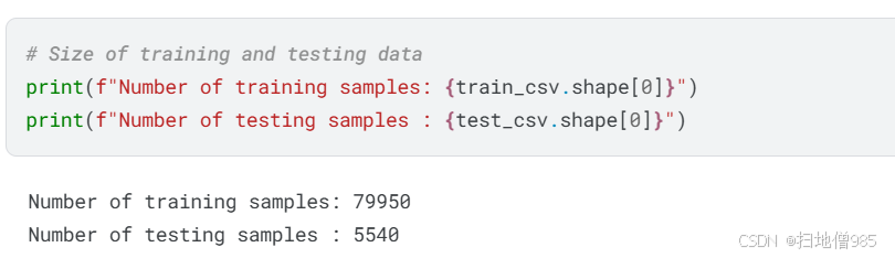
The training dataset consists of approximately 80,000 images, which provides a substantial amount of data for training an AI model to distinguish between AI-generated and human-created images. This large dataset helps the model learn important features for classification.

The testing dataset contains around 5,500 images, which is also a reasonable size. However, these images do not have true labels, meaning they cannot be used for standard model evaluation. Instead, they serve as inference data rather than traditional test data.

To ensure proper model evaluation and prevent overfitting, the training dataset should be split into three subsets:

Training Data – Used to train the model.
Validation Data – Used to tune hyperparameters and monitor performance.
Testing Data – A separate labeled set for final evaluation (if available).

Since the provided test images lack labels, a portion of the training data should be set aside for validation and testing purposes.

# Compute Class Distribution
class_dis = train_csv.label.value_counts().reset_index()

# Visualization
pie_fig = px.pie(
    class_dis,
    names='label',
    values='count',
    title='Class Distribution',
    hole=0.2,
)
pie_fig.show()

bar_fig = px.bar(
    class_dis,
    x='label',
    y='count',
    title='Class Distribution',
    text='count'
)
bar_fig.update_layout(
    xaxis_title='Label',
    yaxis_title='Frequency Count'
)
bar_fig.show()

数据集平衡性

该数据集具有平衡的类别分布，每个类别大约有40,000张图像，从而实现AI生成图像与人类创作图像之间50-50%的平衡分配。

这种平衡性是有益的，因为：

无类别不平衡问题——我们无需应用过采样或欠采样等技术。
平等的学习机会——模型将平等地学习两个类别，从而降低产生偏差的风险。
预处理简化——无需进行额外的调整来纠正类别分布。

由于数据分布均匀，因此可以在不担心类别不平衡影响性能的情况下有效地训练模型。

数据加载

既然我们已经了解了数据集的结构，下一步就是加载数据。

一个重要的观察结果是，这些图像的形状各异——有些图像高度横向拉伸，而其他图像则更偏向纵向。这意味着它们的长宽比不同，呈现为矩形而非统一的正方形。

无论是用于训练还是推理，图像都需要被调整为一致的形状。尽管调整大小可能会稍微扭曲某些图像并改变其原始结构，但这是确保与深度学习模型兼容所必需的，因为深度学习模型需要固定的输入维度。

各种调整大小的技术，如裁剪、填充或保持长宽比的调整大小，可以在保持分类重要特征的同时，帮助最小化失真。

for i in range(10):
    shape = plt.imread(f'{main_dir}/{train_csv.file_name[i]}').shape
    print(f"Shape of the Image: {shape}")

Shape of the Image: (768, 512, 3)
Shape of the Image: (768, 512, 3)
Shape of the Image: (512, 768, 3)
Shape of the Image: (512, 768, 3)
Shape of the Image: (768, 512, 3)
Shape of the Image: (768, 512, 3)
Shape of the Image: (512, 768, 3)
Shape of the Image: (512, 768, 3)
Shape of the Image: (528, 768, 3)
Shape of the Image: (528, 768, 3)

分析数据集时，我们观察到图像的大小各异，常见的尺寸约为500×1000或500×800像素。

为了使这些图像与我们的模型兼容，我们需要将它们调整为标准形状。深度学习模型常见的选择包括256×256、224×224、512×512或1024×1024像素。

由于1024×1024的图像较大，可能会增加计算成本，因此我们将从更易于管理的尺寸开始，例如512×512。如果这种分辨率不能产生令人满意的结果，我们可以尝试更大的尺寸，如1024×1024，以保留更多细节。

# Collect Training image paths
image_paths, image_labels = train_csv.file_name, train_csv.label
# Define split sizes (80% train, 10% val, 10% test)
total_size = len(image_paths)
train_size = int(0.8 * total_size)
val_size = int(0.1 * total_size)
test_size = int(0.1 * total_size)

print(f"Training Data   : {train_size}")
print(f"Testing Data    : {test_size}")
print(f"Validation Data : {val_size}")

Training Data   : 63960
Testing Data    : 7995
Validation Data : 7995

train_paths, train_labels = image_paths[:train_size], image_labels[:train_size]
val_paths, val_labels = image_paths[train_size:train_size+val_size], image_labels[train_size:train_size+val_size]
test_paths, test_labels = image_paths[train_size+val_size:], image_labels[train_size+val_size:]
BATCH_SIZE = 32

# Updated generator function that works for train, val, and test sets
def image_generator(file_paths, labels):
    for file_path, label in zip(file_paths, labels):
        file_path = main_dir + '/' + file_path
        image = cv2.imread(file_path)  # Read using OpenCV
        image = cv2.cvtColor(image, cv2.COLOR_BGR2RGB)  # Convert to RGB
        image = cv2.resize(image, (512, 512))  # Resize
        image = image.astype(np.float32) / 255.0  # Normalize
        yield image, label  # Yield image and label

# Function to create datasets
def create_dataset(file_paths, labels, batch_size=BATCH_SIZE):
    return tf.data.Dataset.from_generator(
        lambda: image_generator(file_paths, labels),
        output_signature=(
            tf.TensorSpec(shape=(512, 512, 3), dtype=tf.float32),
            tf.TensorSpec(shape=(), dtype=tf.float32)
        )
    ).batch(batch_size).prefetch(tf.data.AUTOTUNE)

# Creating train, validation, and test datasets
train_ds = create_dataset(train_paths, train_labels)
val_ds = create_dataset(val_paths, val_labels)
test_ds = create_dataset(test_paths, test_labels)

既然我们已经将数据划分为训练集、测试集和验证集，我们就可以继续进行模型训练了。然而，在深入训练过程之前，让我们花点时间检查一下数据集中的一些图像。此外，我们可以创建一些辅助函数，以帮助可视化训练过程和数据。

数据可视化

def show_images(data, n_rows=3, n_cols=5, figsize=(15, 10)):
    # Get the images and labels
    images, labels = next(iter(data))

    # Create subplots
    plt.figure(figsize=figsize)
    n_image = 0  # Initialize the image index

    # Loop through the grid and plot images
    for i in range(n_rows):
        for j in range(n_cols):
            if n_image < len(images):  # Ensure we don't index beyond the number of images
                plt.subplot(n_rows, n_cols, n_image + 1)
                plt.imshow(images[n_image])  # Display the image
                plt.axis('off')
                plt.title("AI" if labels[n_image].numpy()==1.0 else "Human")  # Convert label to string for display
                n_image += 1

    plt.show()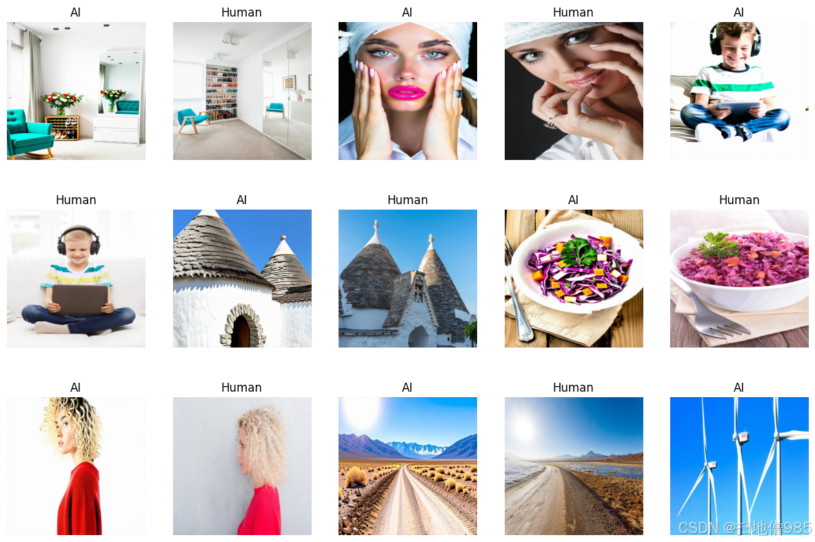

乍一看，很难区分图像是由AI生成还是人类创作的，因为它们往往看起来非常逼真。然而，仔细观察后，一些瑕疵就会显现出来，比如不自然的手势、过分光亮的物体、极端的对比度和亮度，以及清晰度的不规则性。这些技术上的不一致性有助于我们判断图像是由AI生成还是人类创作的。机器学习使我们能够自动化这一过程，而无需手动提取这些特征。通过训练模型，我们可以使它们学习到这些区分特征，并有效地将图像分类为AI生成或人类创作。

预训练模型

既然我们已经对数据进行了可视化和预处理，接下来就该构建深度学习模型了。为了避免从头开始训练模型（这可能非常耗时），我们将使用预训练模型，并对它们进行微调，或者在权重冻结的情况下使用它们以更快获得结果。我们有多个预训练模型可供选择，如InceptionNet、ResNet、MobileNet、VGG等。为了确定哪个模型效果最好，我们将对每个模型进行约10个轮次（epoch）的训练，比较它们的性能，并选择表现最佳的模型。一旦确定了最佳模型，我们将继续训练或微调它，以提高其准确性。

pre_trained_models = {
    'ResNet50':ResNet50(include_top=False, input_shape=(512, 512, 3)),
    'ResNet50V2':ResNet50V2(include_top=False, input_shape=(512, 512, 3)),
    'Xception':Xception(include_top=False, input_shape=(512, 512, 3)),
    'InceptionV3':InceptionV3(include_top=False, input_shape=(512, 512, 3)),
    'ResNet152':ResNet152(include_top=False, input_shape=(512, 512, 3)),
    'ResNet152V2':ResNet152V2(include_top=False, input_shape=(512, 512, 3)),
    'EfficientNetB3':EfficientNetB3(include_top=False, input_shape=(512, 512, 3)), 
    'EfficientNetB5':EfficientNetB5(include_top=False, input_shape=(512, 512, 3))
}

Downloading data from https://storage.googleapis.com/tensorflow/keras-applications/resnet/resnet50_weights_tf_dim_ordering_tf_kernels_notop.h5
94765736/94765736 ━━━━━━━━━━━━━━━━━━━━ 0s 0us/step
Downloading data from https://storage.googleapis.com/tensorflow/keras-applications/resnet/resnet50v2_weights_tf_dim_ordering_tf_kernels_notop.h5
94668760/94668760 ━━━━━━━━━━━━━━━━━━━━ 0s 0us/step
Downloading data from https://storage.googleapis.com/tensorflow/keras-applications/xception/xception_weights_tf_dim_ordering_tf_kernels_notop.h5
83683744/83683744 ━━━━━━━━━━━━━━━━━━━━ 0s 0us/step
Downloading data from https://storage.googleapis.com/tensorflow/keras-applications/inception_v3/inception_v3_weights_tf_dim_ordering_tf_kernels_notop.h5
87910968/87910968 ━━━━━━━━━━━━━━━━━━━━ 0s 0us/step
Downloading data from https://storage.googleapis.com/tensorflow/keras-applications/resnet/resnet152_weights_tf_dim_ordering_tf_kernels_notop.h5
234698864/234698864 ━━━━━━━━━━━━━━━━━━━━ 1s 0us/step
Downloading data from https://storage.googleapis.com/tensorflow/keras-applications/resnet/resnet152v2_weights_tf_dim_ordering_tf_kernels_notop.h5
234545216/234545216 ━━━━━━━━━━━━━━━━━━━━ 1s 0us/step
Downloading data from https://storage.googleapis.com/keras-applications/efficientnetb3_notop.h5
43941136/43941136 ━━━━━━━━━━━━━━━━━━━━ 0s 0us/step
Downloading data from https://storage.googleapis.com/keras-applications/efficientnetb5_notop.h5
115263384/115263384 ━━━━━━━━━━━━━━━━━━━━ 0s 0us/step

if os.path.exists(history_df_path):
    history_df = pd.read_csv(history_df_path, index_col=0)
else:
    histories = {}
    for model_name in pre_trained_models:
        model = pre_trained_models[model_name]
        print(f"Utilizing : {model_name}")
    
        # Freeze Model Weights
        model.trainable = False
    
        # Create another model
        base_model = keras.Sequential([
            model,
            keras.layers.GlobalAveragePooling2D(),
            keras.layers.Dropout(0.4),
            keras.layers.Dense(32, activation='relu'),
            keras.layers.Dense(1, activation='sigmoid')
        ])
    
        # Compile the model
        base_model.compile(
            loss='binary_crossentropy',
            optimizer='adam',
            metrics=['accuracy']
        )
    
        # Fit the Model on training data
        history = base_model.fit(
            train_ds,
            validation_data=val_ds,
            epochs=10,
        )
        histories[model_name] = history
    
        cls()
        del base_model
        del history
    
    # Convert the History callback into Histories
    for name in histories:
        histories[name] = histories[name].history
    
    # Conver the History in DataFrame
    history_df = pd.DataFrame(histories).T
    history_df = history_df.reset_index()
    history_df = history_df.rename(columns={'index': 'Model'})
    
    # Save to CSV File
    history_df.to_csv('history_df.csv')

Model	accuracy	loss	val_accuracy	val_loss
0	ResNet50	[0.7292500138282776, 0.7940000295639038, 0.810...	[0.5681367516517639, 0.46873384714126587, 0.44...	[0.7820000052452087, 0.7699999809265137, 0.800...	[0.4480898678302765, 0.4659704267978668, 0.431...
1	ResNet50V2	[0.8527500033378601, 0.9110000133514404, 0.914...	[0.33727315068244934, 0.22869886457920074, 0.2...	[0.9240000247955322, 0.9039999842643738, 0.934...	[0.24257208406925201, 0.21950335800647736, 0.1...
2	Xception	[0.8025000095367432, 0.8565000295639038, 0.879...	[0.4657147228717804, 0.3363978862762451, 0.300...	[0.843999981880188, 0.8659999966621399, 0.8700...	[0.3606586158275604, 0.31633031368255615, 0.29...
3	InceptionV3	[0.7777500152587891, 0.8550000190734863, 0.859...	[0.47426196932792664, 0.3432822823524475, 0.32...	[0.8339999914169312, 0.8619999885559082, 0.864...	[0.3731083869934082, 0.3295738399028778, 0.306...
4	ResNet152	[0.7582499980926514, 0.8040000200271606, 0.803...	[0.5086648464202881, 0.4455946683883667, 0.442...	[0.7940000295639038, 0.7940000295639038, 0.797...	[0.44360145926475525, 0.4322607219219208, 0.42...
5	ResNet152V2	[0.8582500219345093, 0.9112499952316284, 0.925...	[0.33524543046951294, 0.2287691980600357, 0.19...	[0.9039999842643738, 0.9139999747276306, 0.907...	[0.2537347674369812, 0.21231001615524292, 0.21...
6	EfficientNetB3	[0.5174999833106995, 0.5529999732971191, 0.541...	[0.6935126781463623, 0.6850593090057373, 0.688...	[0.6660000085830688, 0.6700000166893005, 0.671...	[0.6855514645576477, 0.6791845560073853, 0.677...
7	EfficientNetB5	[0.565500020980835, 0.5912500023841858, 0.6052...	[0.6811910271644592, 0.6735778450965881, 0.669...	[0.6800000071525574, 0.7179999947547913, 0.695...	[0.6548061370849609, 0.6500796675682068, 0.648...

既然我们已经训练了模型并记录了它们的训练历史，我们就可以通过绘制结果来分析它们的性能。我们的目标是找出即使训练数据和轮次有限也能表现良好的模型。我们对每个模型进行了八个轮次的训练，让它们自由学习。如果一个模型在这么短的训练时间内就表现出色，那么这就表明它非常适合区分AI生成的图像和人类创作的图像。在这种情况下，我们可以继续对表现最佳的模型进行微调，而不是从头开始构建一个新的模型。

# Get the model names
model_names = history_df.Model

for name in model_names:

    # Get the required data
    data = history_df[history_df.Model == name]

    # Plotting the curve
    plt.figure(figsize=(15,5))
    plt.title(f'{name} - Accuracy Curve')
    plt.plot(eval(data['accuracy'].values[0]), label='Accuracy')
    plt.plot(eval(data['val_accuracy'].values[0]), label='Val Accuracy')
    plt.xlabel('Epochs')
    plt.ylabel('Accuracy')
    plt.legend()
    plt.grid()
    plt.show()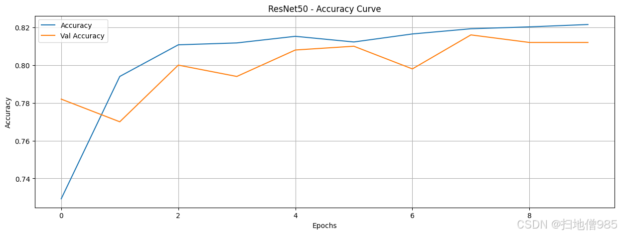

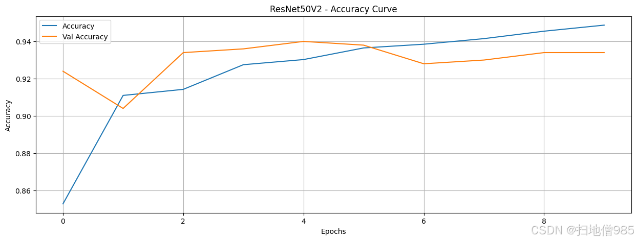
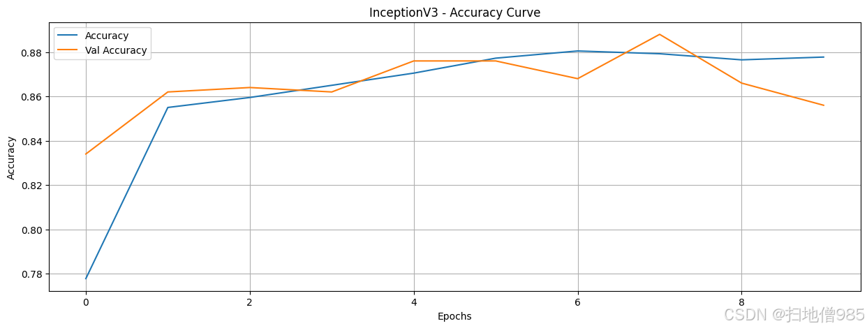
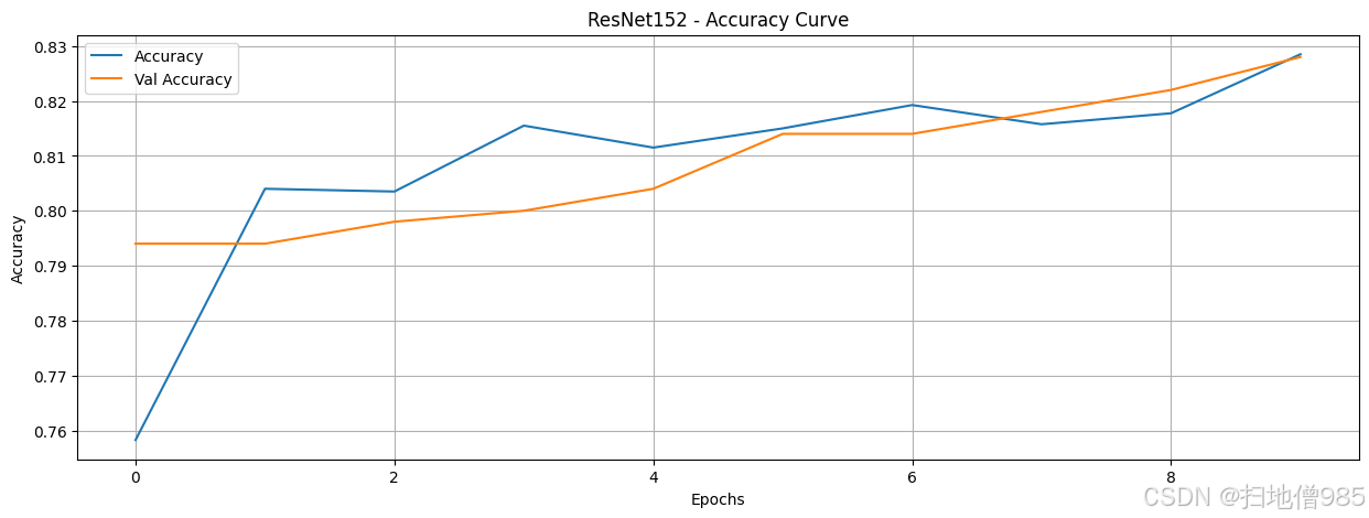
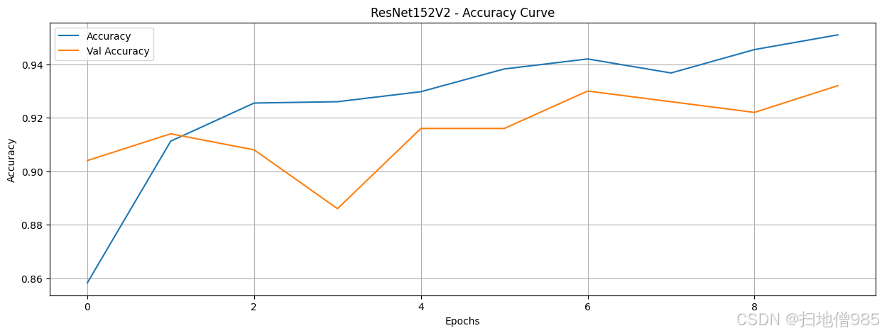
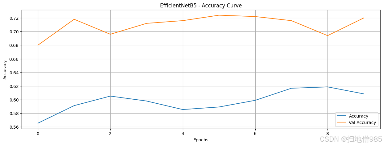
在绘制了包括训练和验证准确率在内的所有模型的准确率曲线后，我们现在可以比较它们的性能。为了简化分析流程，我们不必评估所有模型，而可以只关注那些准确率超过90%的模型。这样做可以让我们更有效地识别出最有前景的模型。然而，仅仅获得高准确率是不够的，我们还需要评估模型的鲁棒性，以确保它们具有良好的泛化能力，并没有过拟合训练数据。