RL(Chapter 5): Monte Carlo Methods (MC) (蒙特卡洛方法)

本文为强化学习笔记，主要参考以下内容：

• Reinforcement Learning: An Introduction
• 代码全部来自 GitHub
• 习题答案参考 Github

Monte Carlo Methods

• Monte Carlo methods are ways of solving the reinforcement learning problem based on averaging sample returns, thus requiring only $experience$—sample sequences of states, actions, and rewards from $actual$ or $simulated$ interaction with an environment. (does not assume complete knowledge of the environment)
  • Of course, if there are very many states, then it may not be practical to keep separate averages for each state individually. Instead, the agent would have to maintain $v_{\pi }$ and $q_{\pi }$ as parameterized functions and adjust the parameters to better match the observed returns. This can also produce accurate estimates.

Here we use the term “Monte Carlo” specifically for methods based on averaging $complete$ returns, as opposed to methods that learn from partial returns, considered in the next chapter.

• Here we define Monte Carlo methods only for episodic tasks. Only on the completion of an episode are value estimates and policies changed. Monte Carlo methods can thus be incremental in an episode-by-episode sense, but not in a step-by-step (online) sense.

---

• Monte Carlo methods sample and average $returns$ for each state–action pair much like the bandit methods we explored in Chapter 2. The main difference is that now there are multiple states, each acting like a different bandit problem (like an associative-search or contextual bandit) and the different bandit problems are interrelated. That is, the return after taking an action in one state depends on the actions taken in later states in the same episode. Because all the action selections are undergoing learning, the problem becomes nonstationary.
• To handle the nonstationarity, we adapt the idea of general policy iteration (GPI). Whereas in DP we $computed$ value functions from knowledge of the MDP, here we $learn$ value functions from sample returns with the MDP. The value functions and corresponding policies still interact to attain optimality in essentially the same way (GPI).

Monte Carlo Prediction

• We begin by considering Monte Carlo methods for learning the state-value function for a given policy.
  
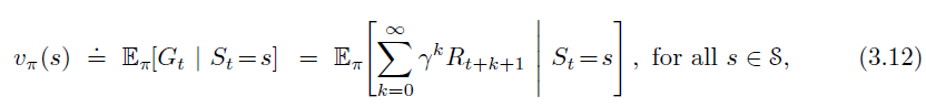
• An obvious way to estimate it from experience, then, is simply to average the returns observed after visits to that state.

由强大数定理可知，采样均值以概率 1 收敛于均值

---

• In particular, suppose we wish to estimate $v_{\pi }(s)$, given a set of episodes obtained by following $\pi$ and passing through $s$. Each occurrence of state $s$ in an episode is called a $visit$ to $s$. Let us call the first time it is visited in an episode the $first$ $visit$ to $s$.
  • The $first$-$visit$ MC $method$ (首次访问型 MC 算法) estimates $v_{\pi }(s)$ as the average of the returns following first visits to $s$
  • The $every$-$visit$ MC $method$ (每次访问型 MC 算法) averages the returns following all visits to $s$
• These two Monte Carlo (MC) methods are very similar but have slightly different theoretical properties. First-visit MC has been most widely studied, and is the one we focus on in this chapter. Every-visit MC extends more naturally to function approximation and eligibility traces (资格迹).
• Both first-visit MC and every-visit MC converge to $v_{\pi }(s)$ as the number of visits (or first visits) to $s$ goes to infinity.
  • This is easy to see for the case of first-visit MC. In this case each return is an independent, identically distributed estimate of $v_{\pi }(s)$ with finite variance. By the law of large numbers the sequence of averages of these estimates converges to their expected value.
  • Every-visit MC is less straightforward, but its estimates also converge quadratically (二次收敛) to $v_{\pi }(s)$.

Every-visit MC would be the same except without the check for $S_t$ having occurred earlier in the episode.

---

Differences between $MC$ and $DP:$

Can we generalize the idea of backup diagrams to Monte Carlo algorithms?

• The general idea of a backup diagram is to show at the top the root node to be updated and to show below all the transitions and leaf nodes whose rewards and estimated values contribute to the update.
• For Monte Carlo estimation of $v_{\pi }$, the root is a state node, and below it is the entire trajectory of transitions along a particular single episode, ending at the terminal state, as shown below.
  • Whereas the DP diagram shows all possible transitions, the Monte Carlo diagram shows only those sampled on the one episode.
  • Whereas the DP diagram includes only one-step transitions, the Monte Carlo diagram goes all the way to the end of the episode.
    

---

Monte Carlo methods do not $bootstrap$ (自举)

• An important fact about Monte Carlo methods is that the estimates for each state are independent. The estimate for one state does not build upon the estimate of any other state, as is the case in $DP$. In other words, Monte Carlo methods do not $bootstrap$.
• In particular, note that the computational expense of estimating the value of a single state is independent of the number of states.
  • This can make Monte Carlo methods particularly attractive when one requires the value of only one or a subset of states. One can generate many sample episodes starting from the states of interest, averaging returns from only these states, ignoring all others.

This is a third advantage Monte Carlo methods can have over DP methods (after the ability to learn from actual experience and from simulated experience).

Monte Carlo Estimation of Action Values

If a model is not available, then it is particularly useful to estimate $action$ values (the values of state–action pairs) rather than $state$ values.

• With a model, state values alone are sufficient to determine a policy; (greedy policy is the optimal policy)
• Without a model, however, state values alone are not sufficient. One must explicitly estimate the value of each action in order for the values to be useful in suggesting a policy.

Thus, one of our primary goals for Monte Carlo methods is to estimate $q_{\ast }$.

如果只知道 $v_{\ast }(s)$ 的话，要想求出最优策略，根据贝尔曼方程，必须找到使 $q_{\ast }(s,a)=v_{\ast }(s)$ 的动作

---

• The policy evaluation problem for action values is to estimate $q_{\pi }(s,a)$, the expected return when starting in state $s$, taking action $a$, and thereafter following policy $\pi$.
• The Monte Carlo methods for this are essentially the same as just presented for state values, except now we talk about visits to a state–action pair rather than to a state. A state–action pair $s,a$ is said to be visited in an episode if ever the state $s$ is visited and action $a$ is taken in it.
  • every-visit MC
  • first-visit MC

---

• The only complication is that many state–action pairs may never be visited. If $\pi$ is a deterministic policy, then in following $\pi$ one will observe returns only for one of the actions from each state. With no returns to average, the Monte Carlo estimates of the other actions will not improve with experience.

This is the general problem of $maintaining$ $exploration$.

• One way to do this is by specifying that the episodes start in a state–action pair, and that every pair has a nonzero probability of being selected as the start. This guarantees that all state–action pairs will be visited an infinite number of times in the limit of an infinite number of episodes. We call this the assumption of $exploring$ $starts$. (试探性出发)
  • The assumption of exploring starts is sometimes useful, but of course it cannot be relied upon in general, particularly when learning directly from actual interaction with an environment. In that case the starting conditions are unlikely to be so helpful.
• The most common alternative approach is to consider only policies that are stochastic with a nonzero probability of selecting all actions in each state.

For now, we retain the assumption of exploring starts and complete the presentation of a full Monte Carlo control method.

Monte Carlo Control

Use Monte Carlo estimation to approximate optimal policies.

The overall idea is to proceed according to the idea of generalized policy iteration (GPI).

• In GPI one maintains both an approximate policy and an approximate value function.
  • The value function is repeatedly altered to more closely approximate the value function for the current policy.
  • The policy is repeatedly improved with respect to the current value function.
    

---

• To begin, let us consider a Monte Carlo version of classical policy iteration.
  where $\stackrel{E}{⟶}$ denotes a complete policy evaluation and $\stackrel{I}{⟶}$ denotes a complete policy improvement.
• Policy evaluation is done exactly as described in the preceding section. Many episodes are experienced, with the approximate action-value function approaching the true function asymptotically.
  • For the moment, let us assume that we do indeed observe an infinite number of episodes and that, in addition, the episodes are generated with exploring starts.
  • Under these assumptions, the Monte Carlo methods will compute each $q_{{\pi }_k}$ exactly, for arbitrary ${\pi }_k$.
• Policy improvement is done by making the policy greedy with respect to the current action-value function $q$:
  According to $\mathbf{p}\mathbf{o}\mathbf{l}\mathbf{i}\mathbf{c}\mathbf{y}$ $\mathbf{i}\mathbf{m}\mathbf{p}\mathbf{r}\mathbf{o}\mathbf{v}\mathbf{e}\mathbf{m}\mathbf{e}\mathbf{n}\mathbf{t}$ $\mathbf{t}\mathbf{h}\mathbf{e}\mathbf{o}\mathbf{r}\mathbf{e}\mathbf{m}$, we have $v_{{\pi }_{k+1}}(s)\ge v_{{\pi }_k}(s).$ (proved here)
• In this way Monte Carlo methods can be used to find optimal policies given only sample episodes and no other knowledge of the environment’s dynamics.

---

• We made two unlikely assumptions above in order to easily obtain this guarantee of convergence for the Monte Carlo method.
  • One was that the episodes have exploring starts.
  • The other was that policy evaluation could be done with an infinite number of episodes.
• To obtain a practical algorithm we will have to remove both assumptions.

For now we focus on the second assumption, which is relatively easy to remove. There are two ways to solve the problem.

• One is to hold firm to the idea of approximating $q_{{\pi }_k}$ in each policy evaluation.
  • Measurements and assumptions are made to obtain bounds on the magnitude and probability of error in the estimates, and then sufficient steps are taken during each policy evaluation to assure that these bounds are sufficiently small.
  • This approach can probably be made completely satisfactory in the sense of guaranteeing correct convergence up to some level of approximation. However, it is also likely to require far too many episodes to be useful in practice on any but the smallest problems.
• A second approach to avoiding the infinite number of episodes nominally required for policy evaluation, in which we give up trying to complete policy evaluation before returning to policy improvement. On each evaluation step we move the value function toward $q_{{\pi }_k}$ , but we do not expect to actually get close except over many steps.
  • One extreme form of the idea is value iteration, in which only one iteration of iterative policy evaluation is performed between each step of policy improvement. The in-place version of value iteration is even more extreme; there we alternate between improvement and evaluation steps for single states.

For Monte Carlo policy iteration it is natural to alternate between evaluation and improvement on an episode-by-episode basis.

• After each episode, the observed returns are used for policy evaluation, and then the policy is improved at all the states visited in the episode.

$Q(S_t,A_t)\leftarrow average(Returns(S_t,A_t))$ can be replaced by incremental implementation.

Monte Carlo Control without Exploring Starts (On-Policy)

• $On$-$policy$ methods (同轨策略)
  • On-policy methods attempt to evaluate or improve the policy that is used to make decisions.
  • e.g. Monte Carlo ES Method
• $Off$-$policy$ methods (离轨策略)
  • Off-policy methods evaluate or improve a policy different from that used to generate the data.

---

$\epsilon$-$soft$ policies

• In on-policy control methods the policy is generally $soft$, meaning that $\pi (a|s)>0$ for all $s\in \mathcal{S}$ and all $a\in \mathcal{A}(s)$, but gradually shifted closer and closer to a deterministic optimal policy.
  • The on-policy method we present in this section uses $\epsilon$-greedy policies. That is, all nongreedy actions are given the minimal probability of selection, $\frac{\epsilon }{|\mathcal{A}(s)|}$, and the remaining bulk of the probability, $1-\epsilon +\frac{\epsilon }{|\mathcal{A}(s)|}$, is given to the greedy action.
  • The $\epsilon$-greedy policies are examples of $\epsilon$-$soft$ policies, defined as policies for which $\pi (a|s)\ge \frac{ϵ}{|\mathcal{A}(s)|}$ for all states and actions.

soft policy 很好地替代了 exploring starts 的苛刻条件

---

• The overall idea of on-policy Monte Carlo control is still that of GPI. Fortunately, GPI does not require that the policy be taken all the way to a greedy policy, only that it be moved toward a greedy policy. The discussion below shows that policy iteration works for $\epsilon$-soft policies.
• That any $\epsilon$-greedy policy with respect to $q_{\pi }$ is an improvement over any $\epsilon$-soft policy $\pi$ is assured by the policy improvement theorem. Let ${\pi }^{\prime }$ be the $\epsilon$-greedy policy.
  (the sum is a weighted average with nonnegative weights summing to 1, and as such it must be less than or equal to the largest number averaged)
  Thus, by the policy improvement theorem, ${\pi }^{\prime }\ge \pi$.
• We now prove that equality can hold only when both ${\pi }^{\prime }$ and $\pi$ are optimal among the $\epsilon$-soft policies.
  • Consider a new environment that is just like the original environment, except with the requirement that policies be $\epsilon$-soft “moved inside” the environment. The new environment has the same action and state set as the original and behaves as follows:
    • If in state $s$ and taking action $a$, then with probability $1-\epsilon$ the new environment behaves exactly like the old environment. With probability $\epsilon$ it repicks the action at random, with equal probabilities, and then behaves like the old environment with the new, random action.
  • The best one can do in this new environment with general policies is the same as the best one could do in the original environment with $\epsilon$-soft policies.
  • Let ${\tilde{v}}_{\ast }$ and ${\tilde{q}}_{\ast }$ denote the optimal value functions for the new environment. Then a policy $\pi$ is optimal among $\epsilon$-soft policies if and only if $v_{\pi }$ = ${\tilde{v}}_{\ast }$. From the definition of ${\tilde{v}}_{\ast }$ we know that it is the unique solution to
    When equality holds and the $\epsilon$-soft policy $\pi$ is no longer improved, then we also know, from (5.2), that
    However, this equation is the same as the previous one, except for the substitution of $v_{\pi }$ for ${\tilde{v}}_{\ast }$. Because ${\tilde{v}}_{\ast }$ is the unique solution, it must be that $v_{\pi }={\tilde{v}}_{\ast }$.

Off-policy Prediction via Importance Sampling

All learning control methods face a dilemma:

• They seek to learn action values conditional on subsequent optimal behavior (exploit), but they need to behave non-optimally in order to explore all actions.

How can they learn about the optimal policy while behaving according to an exploratory policy?

• The on-policy approach in the preceding section is actually a compromise—it learns action values not for the optimal policy, but for a near-optimal policy that still explores.

---

A more straightforward approach is to use two policies,

• one is learned about and becomes the optimal policy (target policy (目标策略))
• one is more exploratory and is used to generate behavior. (behavior policy (行动策略))
• In this case we say that learning is from data “off” the target policy, and the overall process is termed $off$-$policy$ learning.

---

• Because the data is due to a different policy, off-policy methods are often of greater variance and are slower to converge.
• On the other hand, off-policy methods are more powerful and general. They include on-policy methods as the special case in which the target and behavior policies are the same.

---

Prediction problem

In this section, we consider the prediction problem, in which $\pi$ is unchanging and given.

• Suppose we wish to estimate $v_{\pi }$ or $q_{\pi }$, but all we have are episodes following another policy $b$, where $b\ne \pi$.
  • In this case, $\pi$ is the target policy, $b$ is the behavior policy, and both policies are considered fixed and given. (Often, $\pi$ is the greedy policy and $b$ is a more exploratory policy, perhaps $\epsilon$-greedy)
• the assumption of $coverage$ (覆盖假设)
  • In order to use episodes from $b$ to estimate values for $\pi$, we require that every action taken under $\pi$ is also taken, at least occasionally, under $b$. That is, we require that $\pi (a|s)>0$ implies $b(a|s)>0$.
  • It follows from coverage that $b$ must be stochastic in states where it is not identical to $\pi$.
• The target policy $\pi$ may be deterministic, and, in fact, this is a case of particular interest in control applications.
  • In control, the target policy is typically the deterministic greedy policy with respect to the current estimate of the action-value function. This policy becomes a deterministic optimal policy while the behavior policy remains stochastic and more exploratory, for example, an $\epsilon$-greedy policy.

---

Importance sampling

• Almost all off-policy methods utilize importance sampling, a general technique for estimating expected values under one distribution given samples from another.
• We apply importance sampling to off-policy learning by weighting returns according to the relative probability of their trajectories occurring under the target and behavior policies, called the $\mathbf{i}\mathbf{m}\mathbf{p}\mathbf{o}\mathbf{r}\mathbf{t}\mathbf{a}\mathbf{n}\mathbf{c}\mathbf{e}$-$\mathbf{s}\mathbf{a}\mathbf{m}\mathbf{p}\mathbf{l}\mathbf{i}\mathbf{n}\mathbf{g}$ $\mathbf{r}\mathbf{a}\mathbf{t}\mathbf{i}\mathbf{o}$ (重要度采样比).
  • Given a starting state $S_t$, the probability of the subsequent state–action trajectory, $A_t,S_{t+1},A_{t+1},...,S_T$ , occurring under any policy $\pi$ is
    
  • Thus, the importance-sampling ratio is
    The importance sampling ratio ends up depending only on the two policies and the sequence, not on the MDP.
• Recall that we wish to estimate the expected returns (values) under the target policy, but all we have are returns $G_t$ due to the behavior policy. These returns have the wrong expectation $\mathbb{E}[G_t|S_t=s]=v_b(s)$ and so cannot be averaged to obtain $v_{\pi }$. This is where importance sampling comes in. The ratio ${\rho }_{t:T-1}$ transforms the returns to have the right expected value:
  
  • For example, if any one of the actions would never be taken by $\pi$ (i.e., $\pi (A_k|S_k)=0$) then the return should be given zero weight and be totally ignored.
  • On the other hand, if by chance an action is taken that $\pi$ would take with much greater probability than $b$ does, then this will increase the weight that would otherwise be given to the return. This makes sense because that action is characteristic of $\pi$ (and therefore we want to learn about it) but is selected only rarely by $b$ and thus rarely appears in the data. To make up for this we have to over-weight it when it does occur.
  • Note that if the two policies are actually the same (the on-policy case) then the importance sampling ratio is always 1. Thus our new update generalizes the previous on-policy version.

This is intuitively right, but can this be proved mathematically?

---

Now we are ready to give a Monte Carlo algorithm that averages returns from a batch of observed episodes following policy $b$ to estimate $v_{\pi }(s)$.

• It is convenient here to number time steps in a way that increases across episode boundaries.
  • That is, if the first episode of the batch ends in a terminal state at time 100, then the next episode begins at time $t=101$. This enables us to use time-step numbers to refer to particular steps in particular episodes.
• In particular, we can define the set of all time steps in which state $s$ is visited, denoted $\mathcal{T}(s)$. This is for an every-visit method; for a first-visit method, $\mathcal{T}(s)$ would only include time steps that were first visits to $s$ within their episodes.
• Also, let $T(t)$ denote the first time of termination following time $t$, and $G_t$ denote the return after $t$ up through $T(t)$. Then { G t } t ∈ T ( s ) \{G_t\}_{t\in\mathcal T(s)} {Gt​}t∈T(s)​ are the returns that pertain to state $s$, and { ρ t : T ( t ) − 1 } t ∈ T ( s ) \{\rho_{t:T(t)-1}\}_{t\in\mathcal T(s)} {ρt:T(t)−1​}t∈T(s)​ are the corresponding importance-sampling ratios.

Ordinary importance sampling

• To estimate $v_{\pi }(s)$, we simply scale the returns by the ratios and average the results:
  

Weighted importance sampling

• We can also use a $weighted$ $average$, defined as
  or zero if the denominator is zero.

Ordinary VS Weighted importance sampling

• To understand these two varieties of importance sampling, consider the estimates of their first-visit methods after observing a single return from state $s$.
  • In the weighted-average estimate, the ratio ${\rho }_{t:T(t)-1}$ for the single return cancels in the numerator and denominator, so that the estimate is equal to the observed return independent of the ratio (assuming the ratio is nonzero). Given that this return was the only one observed, this is a reasonable estimate, but its expectation is $v_b(s)$ rather than $v_{\pi }(s)$, and in this statistical sense it is biased.
  • In contrast, the first-visit version of the ordinary importance-sampling estimator (5.5) is always $v_{\pi }(s)$ in expectation (it is unbiased), but it can be extreme.
    • Suppose the ratio were ten, indicating that the trajectory observed is ten times as likely under the target policy as under the behavior policy. In this case the ordinary importance-sampling estimate would be ten times the observed return. That is, it would be quite far from the observed return even though the episode’s trajectory is considered very representative of the target policy.
• Formally, the difference between the first-visit methods of the two kinds of importance sampling is expressed in their biases and variances.
  • Ordinary importance sampling is unbiased whereas weighted importance sampling is biased (though the bias converges asymptotically to zero).
  • On the other hand, the variance of ordinary importance sampling is in general unbounded because the variance of the ratios can be unbounded, whereas in the weighted estimator the largest weight on any single return is one.
    • In fact, assuming bounded returns, the variance of the weighted importance-sampling estimator converges to zero even if the variance of the ratios themselves is infinite. In practice, the weighted estimator usually has dramatically lower variance and is strongly preferred.

---

Every-visit methods and First-visit methods

• The every-visit methods for ordinary and weighed importance sampling are both biased, though, again, the bias falls asymptotically to zero as the number of samples increases.
• In practice, every-visit methods are often preferred because they remove the need to keep track of which states have been visited and because they are much easier to extend to approximations.

---

Example 5.5: Infinite Variance

• The estimates of ordinary importance sampling will typically have infinite variance, and thus unsatisfactory convergence properties, whenever the scaled returns have infinite variance—and this can easily happen in off-policy learning when trajectories contain loops.
• A simple example is shown inset in Figure 5.4. There is only one nonterminal state $s$ and two actions, $right$ and $left$. The $right$ action causes a deterministic transition to termination, whereas the left action transitions, with probability 0.9, back to $s$ or, with probability 0.1, on to termination. The rewards are $+1$ on the latter transition and otherwise zero.
• Consider the target policy that always selects left. All episodes under this policy consist of some number (possibly zero) of transitions back to $s$ followed by termination with a reward and return of +1. Thus the value of $s$ under the target policy is 1 ($\gamma =1$).
  
• Suppose we are estimating this value from off-policy data using the behavior policy that selects right and left with equal probability. Even after millions of episodes, the estimates fail to converge to the correct value of 1. In contrast, the weighted importance-sampling algorithm would give an estimate of exactly 1 forever after the first episode that ended with the left action. All returns not equal to 1 (that is, ending with the right action) would be inconsistent with the target policy and thus would have a ${\rho }_{t:T(t)-1}$ of zero and contribute neither to the numerator nor denominator of (5.6). The weighted importance-sampling algorithm produces a weighted average of only the returns consistent with the target policy, and all of these would be exactly 1.
• We can verify that the variance of the importance-sampling-scaled returns is infinite in this example by a simple calculation.
  Thus, if the mean is finite, as it is in our case, the variance is infinite if and only if $\mathbb{E}[X^2]$ is infinite. Thus, we need only show that the expected square of the importance-sampling-scaled return is infinite:
  To compute this expectation, we break it down into cases based on episode length and termination.
  • First note that, for any episode ending with the right action, the importance sampling ratio is zero; these episodes thus contribute nothing to the expectation and can be ignored. We need only consider episodes that involve some number (possibly zero) of left actions that transition back to the nonterminal state, followed by a left action transitioning to termination. All of these episodes have a return of 1, so the $G_0$ factor can be ignored.
  • To get the expected square we need only consider each length of episode, multiplying the probability of the episode’s occurrence by the square of its importance-sampling ratio, and add these up:
    

---

Exercise 5.6

What is the equation analogous to (5.6) for action values $Q(s,a)$ instead of state values $V(s)$, again given returns generated using $b$?

ANSWER

---

Exercise 5.7

In learning curves such as those shown in Figure 5.3 error generally decreases with training, as indeed happened for the ordinary importance-sampling method. But for the weighted importance-sampling method error first increased and then decreased. Why do you think this happened?

ANSWER

• The weighted average algorithm will need few episodes to decrease its bias. Especially when the ${\rho }_{t:T(t)-1}$ is big, the weighted average algorithm would be shifted by those data. When we get enough episodes, the average begins to be stable and decreasing the bias.

---

Exercise 5.8

The results with Example 5.5 and shown in Figure 5.4 used a first-visit MC method. Suppose that instead an every-visit MC method was used on the same problem. Would the variance of the estimator still be infinite? Why or why not?

ANSWER

• For every visit, we have:
  
• On the other hand, considering weighted average method:
  

Incremental Implementation

• Monte Carlo prediction methods can be implemented incrementally, on an episode-by-episode basis. Whereas in Chapter 2 we averaged rewards, in Monte Carlo methods we average $returns$.

---

Ordinary importance sampling

• In ordinary importance sampling, the returns are scaled by the importance sampling ratio ${\rho }_{t:T(t)-1}$, then simply averaged.
• For these methods we can again use the incremental methods.

---

Weighted importance sampling

• Suppose we have a sequence of returns $G_1,G_2,...,G_{n-1}$, all starting in the same state and each with a corresponding random weight $W_i$ (e.g., $W_i={\rho }_{t_i:T(t_i)-1}$). We wish to form the estimate
  and keep it up-to-date as we obtain a single additional return $G_n$. In addition to keeping track of $V_n$, we must maintain for each state the cumulative sum $C_n$ of the weights given to the first $n$ returns. The update rule for $V_n$ is
  and
  where $C_0=0$ (and $V_1$ is arbitrary).

---

The algorithm is nominally for the off-policy case, using weighted importance sampling, but applies as well to the on-policy case just by choosing the target and behavior policies as the same (in which case ($\pi =b$), $W$ is always $1$). The approximation $Q$ converges to $q_{\pi }$ (for all encountered state–action pairs) while actions are selected according to a potentially different policy, $b$.

Off-policy Monte Carlo Control

• Off-policy Monte Carlo control methods follow the behavior policy while learning about and improving the target policy.
  • An advantage of this separation is that the target policy may be deterministic (e.g., greedy), while the behavior policy can continue to sample all possible actions.
• These techniques require that the behavior policy has a nonzero probability of selecting all actions that might be selected by the target policy (coverage assumption). To explore all possibilities, we require that the behavior policy be soft.

---

The box below shows an off-policy Monte Carlo control method, based on GPI and weighted importance sampling, for estimating ${\pi }_{\ast }$ and $q_{\ast }$.

• The target policy $\pi \approx {\pi }_{\ast }$ is the greedy policy with respect to $Q$, which is an estimate of $q_{\pi }$.
• The behavior policy $b$ can be anything, but in order to assure convergence of $\pi$ to the optimal policy, an infinite number of returns must be obtained for each pair of state and action. This can be assured by choosing $b$ to be $\epsilon$-soft.
• The policy $\pi$ converges to optimal at all encountered states even though actions are selected according to a different soft policy $b$, which may change between or even within episodes.

• A potential problem is that this method learns only from the tails of episodes, when all of the remaining actions in the episode are greedy. If nongreedy actions are common, then learning will be slow, particularly for states appearing in the early portions of long episodes. Potentially, this could greatly slow learning.
  • There has been insufficient experience with off-policy Monte Carlo methods to assess how serious this problem is. If it is serious, the most important way to address it is probably by incorporating temporal-difference learning (时序差分学习). Alternatively, if $\gamma$ is less than 1, then the idea developed in the next section may also help significantly.