【第一周】吴恩达团队AI for Medical Diagnosis课程实验

系列文章目录

【第一周】吴恩达团队AI for Medical Diagnosis课程笔记_十三豆腐脑的博客-CSDN博客【第一周】吴恩达团队AI for Medical Diagnosis大作业_十三豆腐脑的博客-CSDN博客【第一周】吴恩达团队AI for Medical Diagnosis课程笔记_十三豆腐脑的博客-CSDN博客

---

目录

系列文章目录

前言

一、数据探索&图像预处理

1.探索

1.1 数据类型和空值检查

1.2 唯一 ID 检查

1.3 数据标签

1.4 数据可视化

 1.5 研究单个图像

1.6 研究像素值分布

2. Keras 中的图像预处理

2.1 标准化

二、计算标签和加权损失函数

1.加权损失函数

1.1 理解加权损失函数

1.2 常规损失函数的问题

1.3 两种模型的加权损失处理

2. 一个以上类别的加权损失

2.1 选择axis=0或axis=1

2.2 计算权重

三、DenseNet

四、患者重叠和数据泄露

1.数据

1.1载入数据

 1.2提取患者ID

 1.3比较训练集和验证集的 PatientID

1.4 识别和移除重叠患者

1.5 健全性检查

---

前言

将课程笔记中实验部分另写一篇。

---

一、数据探索&图像预处理

在本课程的第一个作业中，您将使用从公共 ChestX-ray8 数据集中拍摄的胸部 X 射线图像。 在此笔记本中，您将有机会探索此数据集并熟悉您将在第一次评分作业中使用的一些技术。

在开始为任何机器学习项目编写代码之前，第一步是探索您的数据。 用于分析和操作数据的标准 Python 包是 pandas。

在接下来的两个代码单元中，您将导入 pandas 和一个名为 numpy 的包进行数值操作，然后使用 pandas 将 csv 文件读入数据帧并打印出前几行数据。

# Import necessary packages
import pandas as pd
import numpy as np
import matplotlib.pyplot as plt
%matplotlib inline
import os
import seaborn as sns
sns.set()

1.探索

从csv文件读入数据。

# Read csv file containing training datadata
train_df = pd.read_csv("data/nih/train-small.csv")
# Print first 5 rows
print(f'There are {train_df.shape[0]} rows and {train_df.shape[1]} columns in this data frame')
train_df.head()

There are 1000 rows and 16 columns in this data frame

Out[2]:

	Image	Atelectasis	Cardiomegaly	Consolidation	Edema	Effusion	Emphysema	Fibrosis	Hernia	Infiltration	Mass	Nodule	PatientId	Pleural_Thickening	Pneumonia	Pneumothorax
0	00008270_015.png	0	0	0	0	0	0	0	0	0	0	0	8270	0	0	0
1	00029855_001.png	1	0	0	0	1	0	0	0	1	0	0	29855	0	0	0
2	00001297_000.png	0	0	0	0	0	0	0	0	0	0	0	1297	1	0	0
3	00012359_002.png	0	0	0	0	0	0	0	0	0	0	0	12359	0	0	0
4	00017951_001.png	0	0	0	0	0	0	0	0	1	0	0	17951	0	0	0

查看此 csv 文件中的各个列。 该文件包含胸部 X 射线图像的名称（“图像”列），用 1 和 0 填充的列标识基于每个 X 射线图像给出的诊断。

1.1 数据类型和空值检查

运行下一个单元格以探索每列中存在的数据类型以及数据中是否存在任何空值。

# Look at the data type of each column and whether null values are present
train_df.info()

<class 'pandas.core.frame.DataFrame'>
RangeIndex: 1000 entries, 0 to 999
Data columns (total 16 columns):
Image                 1000 non-null object
Atelectasis           1000 non-null int64
Cardiomegaly          1000 non-null int64
Consolidation         1000 non-null int64
Edema                 1000 non-null int64
Effusion              1000 non-null int64
Emphysema             1000 non-null int64
Fibrosis              1000 non-null int64
Hernia                1000 non-null int64
Infiltration          1000 non-null int64
Mass                  1000 non-null int64
Nodule                1000 non-null int64
PatientId             1000 non-null int64
Pleural_Thickening    1000 non-null int64
Pneumonia             1000 non-null int64
Pneumothorax          1000 non-null int64
dtypes: int64(15), object(1)
memory usage: 125.1+ KB

1.2 唯一 ID 检查

“PatientId”具有每个患者的识别号。 关于这样的医疗数据集，您想了解的一件事是，您是否正在查看某些患者的重复数据，或者每张图像是否代表不同的人。

print(f"The total patient ids are {train_df['PatientId'].count()}, from those the unique ids are {train_df['PatientId'].value_counts().shape[0]} ")

The total patient ids are 1000, from those the unique ids are 928 

如您所见，数据集中唯一患者的数量少于总数，因此必须有一些重叠。 对于有多个记录的患者，您需要确保他们不会同时出现在训练和测试集中，以避免数据泄露。

1.3 数据标签

运行接下来的两个代码单元以创建每个患者状况或疾病名称的列表。

columns = train_df.keys()
columns = list(columns)
print(columns)

['Image', 'Atelectasis', 'Cardiomegaly', 'Consolidation', 'Edema', 'Effusion', 'Emphysema', 'Fibrosis', 'Hernia', 'Infiltration', 'Mass', 'Nodule', 'PatientId', 'Pleural_Thickening', 'Pneumonia', 'Pneumothorax']

# Remove unnecesary elements
columns.remove('Image')
columns.remove('PatientId')
# Get the total classes
print(f"There are {len(columns)} columns of labels for these conditions: {columns}")

There are 14 columns of labels for these conditions: ['Atelectasis', 'Cardiomegaly', 'Consolidation', 'Edema', 'Effusion', 'Emphysema', 'Fibrosis', 'Hernia', 'Infiltration', 'Mass', 'Nodule', 'Pleural_Thickening', 'Pneumonia', 'Pneumothorax']

运行下一个单元格以打印出每个条件的正标签（1）的数量

# Print out the number of positive labels for each class
for column in columns:
    print(f"The class {column} has {train_df[column].sum()} samples")

The class Atelectasis has 106 samples
The class Cardiomegaly has 20 samples
The class Consolidation has 33 samples
The class Edema has 16 samples
The class Effusion has 128 samples
The class Emphysema has 13 samples
The class Fibrosis has 14 samples
The class Hernia has 2 samples
The class Infiltration has 175 samples
The class Mass has 45 samples
The class Nodule has 54 samples
The class Pleural_Thickening has 21 samples
The class Pneumonia has 10 samples
The class Pneumothorax has 38 samples

看看上面每个类中标签的计数。 这看起来像一个平衡的数据集吗？

1.4 数据可视化

使用 csv 文件中列出的图像名称，您可以检索与数据框中的每一行数据关联的图像。

运行下面的单元格以可视化从数据集中随机选择的图像。

# Extract numpy values from Image column in data frame
images = train_df['Image'].values

# Extract 9 random images from it
random_images = [np.random.choice(images) for i in range(9)]

# Location of the image dir
img_dir = 'data/nih/images-small/'

print('Display Random Images')

# Adjust the size of your images
plt.figure(figsize=(20,10))

# Iterate and plot random images
for i in range(9):
    plt.subplot(3, 3, i + 1)
    img = plt.imread(os.path.join(img_dir, random_images[i]))
    plt.imshow(img, cmap='gray')
    plt.axis('off')
    
# Adjust subplot parameters to give specified padding
plt.tight_layout()    

Display Random Images

 1.5 研究单个图像

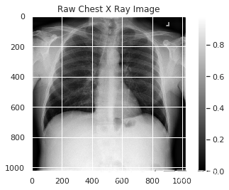
运行下面的单元格以查看数据集中的第一张图像并打印出图像内容的一些详细信息。

# Get the first image that was listed in the train_df dataframe
sample_img = train_df.Image[0]
raw_image = plt.imread(os.path.join(img_dir, sample_img))
plt.imshow(raw_image, cmap='gray')
plt.colorbar()
plt.title('Raw Chest X Ray Image')
print(f"The dimensions of the image are {raw_image.shape[0]} pixels width and {raw_image.shape[1]} pixels height, one single color channel")
print(f"The maximum pixel value is {raw_image.max():.4f} and the minimum is {raw_image.min():.4f}")
print(f"The mean value of the pixels is {raw_image.mean():.4f} and the standard deviation is {raw_image.std():.4f}")

The dimensions of the image are 1024 pixels width and 1024 pixels height, one single color channel
The maximum pixel value is 0.9804 and the minimum is 0.0000
The mean value of the pixels is 0.4796 and the standard deviation is 0.2757

1.6 研究像素值分布

运行下面的单元格以绘制上图中像素值的分布。

# Plot a histogram of the distribution of the pixels
sns.distplot(raw_image.ravel(), 
             label=f'Pixel Mean {np.mean(raw_image):.4f} & Standard Deviation {np.std(raw_image):.4f}', kde=False)
plt.legend(loc='upper center')
plt.title('Distribution of Pixel Intensities in the Image')
plt.xlabel('Pixel Intensity')
plt.ylabel('# Pixels in Image')

Text(0, 0.5, '# Pixels in Image')

2. Keras 中的图像预处理

在训练之前，您将首先修改您的图像，使其更适合训练卷积神经网络。 对于此任务，您将使用 Keras ImageDataGenerator 函数来执行数据预处理和数据增强。

运行接下来的两个单元格以导入此函数并创建一个图像生成器进行预处理。

# Import data generator from keras
from keras.preprocessing.image import ImageDataGenerator

# Normalize images
image_generator = ImageDataGenerator(
    samplewise_center=True, #Set each sample mean to 0.
    samplewise_std_normalization= True # Divide each input by its standard deviation
)

2.1 标准化

您在上面创建的 image_generator 将调整您的图像数据，使数据的新平均值为零，数据的标准差为 1。

换句话说，生成器会将图像中的每个像素值替换为通过减去均值并除以标准差而计算出的新值。
 
运行下一个单元格以使用 image_generator 预处理您的数据。 在此步骤中，您还将图像尺寸减小到 320x320 像素。

# Flow from directory with specified batch size and target image size
generator = image_generator.flow_from_dataframe(
        dataframe=train_df,
        directory="data/nih/images-small/",
        x_col="Image", # features
        # Let's say we build a model for mass detection
        y_col= ['Mass'], # labels
        class_mode="raw", # 'Mass' column should be in train_df
        batch_size= 1, # images per batch
        shuffle=False, # shuffle the rows or not
        target_size=(320,320) # width and height of output image
)

Found 1000 validated image filenames.

运行下一个单元格以绘制预处理图像的示例

# Plot a processed image
sns.set_style("white")
generated_image, label = generator.__getitem__(0)
plt.imshow(generated_image[0], cmap='gray')
plt.colorbar()
plt.title('Raw Chest X Ray Image')
print(f"The dimensions of the image are {generated_image.shape[1]} pixels width and {generated_image.shape[2]} pixels height")
print(f"The maximum pixel value is {generated_image.max():.4f} and the minimum is {generated_image.min():.4f}")
print(f"The mean value of the pixels is {generated_image.mean():.4f} and the standard deviation is {generated_image.std():.4f}")

Clipping input data to the valid range for imshow with RGB data ([0..1] for floats or [0..255] for integers).

The dimensions of the image are 320 pixels width and 320 pixels height
The maximum pixel value is 1.7999 and the minimum is -1.7404
The mean value of the pixels is 0.0000 and the standard deviation is 1.0000

运行下面的单元格以查看新预处理图像与原始图像中像素值分布的比较。

# Include a histogram of the distribution of the pixels
sns.set()
plt.figure(figsize=(10, 7))

# Plot histogram for original iamge
sns.distplot(raw_image.ravel(), 
             label=f'Original Image: mean {np.mean(raw_image):.4f} - Standard Deviation {np.std(raw_image):.4f} \n '
             f'Min pixel value {np.min(raw_image):.4} - Max pixel value {np.max(raw_image):.4}',
             color='blue', 
             kde=False)

# Plot histogram for generated image
sns.distplot(generated_image[0].ravel(), 
             label=f'Generated Image: mean {np.mean(generated_image[0]):.4f} - Standard Deviation {np.std(generated_image[0]):.4f} \n'
             f'Min pixel value {np.min(generated_image[0]):.4} - Max pixel value {np.max(generated_image[0]):.4}', 
             color='red', 
             kde=False)

# Place legends
plt.legend()
plt.title('Distribution of Pixel Intensities in the Image')
plt.xlabel('Pixel Intensity')
plt.ylabel('# Pixel')

Text(0, 0.5, '# Pixel')

这就是本练习的内容，您现在应该更加熟悉您将在本周作业中使用的数据集！ 

二、计算标签和加权损失函数

正如您在讲座视频中看到的，避免类不平衡影响损失函数的一种方法是对损失进行不同的加权。 要选择权重，您首先需要计算类频率。

对于本练习，您将只获得每个标签的计数。 稍后，您将使用此处练习的概念来计算作业中的频率！

# Import the necessary packages
import numpy as np
import pandas as pd
import seaborn as sns
import matplotlib.pyplot as plt
%matplotlib inline

# Read csv file containing training datadata
train_df = pd.read_csv("data/nih/train-small.csv")

# Count up the number of instances of each class (drop non-class columns from the counts)
class_counts = train_df.sum().drop(['Image','PatientId'])

for column in class_counts.keys():
    print(f"The class {column} has {train_df[column].sum()} samples")

The class Atelectasis has 106 samples
The class Cardiomegaly has 20 samples
The class Consolidation has 33 samples
The class Edema has 16 samples
The class Effusion has 128 samples
The class Emphysema has 13 samples
The class Fibrosis has 14 samples
The class Hernia has 2 samples
The class Infiltration has 175 samples
The class Mass has 45 samples
The class Nodule has 54 samples
The class Pleural_Thickening has 21 samples
The class Pneumonia has 10 samples
The class Pneumothorax has 38 samples

# Plot up the distribution of counts
sns.barplot(class_counts.values, class_counts.index, color='b')
plt.title('Distribution of Classes for Training Dataset', fontsize=15)
plt.xlabel('Number of Patients', fontsize=15)
plt.ylabel('Diseases', fontsize=15)
plt.show()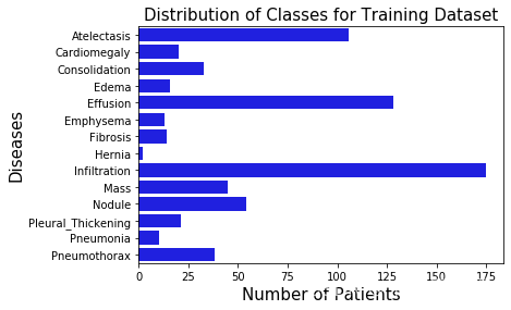

1.加权损失函数

下面是一个计算加权损失的例子。 在作业中，您将计算加权损失函数。 此示例代码将使您对加权损失函数的作用有一些直觉，并帮助您练习将在评分作业中使用的一些语法。

对于此示例，您将首先定义一组假设的真实标签，然后定义一组预测。

运行下一个单元格以创建“ground truth”标签。

# Generate an array of 4 binary label values, 3 positive and 1 negative
y_true = np.array(
        [[1],
         [1],
         [1],
         [0]])
print(f"y_true: \n{y_true}")

y_true: 
[[1]
 [1]
 [1]
 [0]]

1.1 理解加权损失函数

1.1.1 两种模式
为了更好地理解损失函数，您将假设您有两个模型。

对于给出的任何示例，模型 1 始终输出 0.9。
对于给出的任何示例，模型 2 始终输出 0.1。

# Make model predictions that are always 0.9 for all examples
y_pred_1 = 0.9 * np.ones(y_true.shape)
print(f"y_pred_1: \n{y_pred_1}")
print()
y_pred_2 = 0.1 * np.ones(y_true.shape)
print(f"y_pred_2: \n{y_pred_2}")

y_pred_1: 
[[0.9]
 [0.9]
 [0.9]
 [0.9]]

y_pred_2: 
[[0.1]
 [0.1]
 [0.1]
 [0.1]]

1.2 常规损失函数的问题

这里的学习目标是注意到，对于常规损失函数（不是加权损失），始终输出 0.9 的模型比模型 2 的损失更小（性能更好）。

这是因为存在类别不平衡，其中 4 个标签中有 3 个是 1。
如果数据完全平衡（两个标签为 1，两个标签为 0），模型 1 和模型 2 的损失相同。 每个人都会得到两个正确的例子和两个不正确的例子。

但是，由于数据不平衡，因此常规损失函数意味着模型 1 优于模型 2。

1.2.1 常规非加权损失的缺点
看看你从这两个模型中得到了什么损失（模型 1 总是预测 0.9，模型 2 总是预测 0.1），看看每个模型的常规（未加权）损失函数是什么。

loss_reg_1 = -1 * np.sum(y_true * np.log(y_pred_1)) + \
                -1 * np.sum((1 - y_true) * np.log(1 - y_pred_1))
print(f"loss_reg_1: {loss_reg_1:.4f}")


loss_reg_2 = -1 * np.sum(y_true * np.log(y_pred_2)) + \
                -1 * np.sum((1 - y_true) * np.log(1 - y_pred_2))
print(f"loss_reg_2: {loss_reg_2:.4f}")

print(f"When the model 1 always predicts 0.9, the regular loss is {loss_reg_1:.4f}")
print(f"When the model 2 always predicts 0.1, the regular loss is {loss_reg_2:.4f}")

loss_reg_1: 2.6187

loss_reg_2: 7.0131

When the model 1 always predicts 0.9, the regular loss is 2.6187
When the model 2 always predicts 0.1, the regular loss is 7.0131

请注意，当预测始终为 0.1 时，损失函数会产生更大的损失，因为数据不平衡，并且具有三个 1 的标签，但只有一个 0 的标签。

给定具有更多正标签的类不平衡，常规损失函数意味着具有较高预测 0.9 的模型比具有较低预测 0.1 的模型表现更好。

1.3 两种模型的加权损失处理

使用加权损失函数，当预测全部为 0.9 与预测全部为 0.1 时，您将获得相同的加权损失。

请注意 0.9 的预测如何与 1 的正标签相差 0.1。
还要注意 0.1 的预测如何与 0 的负标签相差 0.1
因此，如果将模型 1 和 2 绘制在 0 和 1 之间的数轴上，则模型 1 和 2 沿 0.5 的中点是“对称的”。
 

1.3.1 加权损失方程
计算第零个标签的损失（索引 0 处的列）

损失由两项组成。为了更容易阅读代码，您将分别计算这些术语中的每一个。出于解释的目的，我们为这两个术语中的每一个命名，但这些术语并未正式称为 losspos 或 lossneg
losspos ：我们将使用它来指代实际标签为正的损失（正示例）
lossneg ：我们将使用它来指代实际标签为负的损失（负示例）

由于这个样本数据集足够小，您可以计算要在加权损失函数中使用的正权重。 要获得正权重，请计算存在多少个 NEGATIVE 标签，除以示例总数。

在这种情况下，有一个否定标签，总共有四个示例。

同样，负权重是正标签的比例。

运行下一个单元格来定义正负权重。

# calculate the positive weight as the fraction of negative labels
w_p = 1/4

# calculate the negative weight as the fraction of positive labels
w_n = 3/4

print(f"positive weight w_p: {w_p}")
print(f"negative weight w_n {w_n}")

positive weight w_p: 0.25
negative weight w_n 0.75

1.3.2 加权损失：模型 1
运行接下来的两个单元格分别计算两个损失项。

在这里，loss_1_pos 和 loss_1_neg 是使用 y_pred_1 预测计算的。

# Calculate and print out the first term in the loss function, which we are calling 'loss_pos'
loss_1_pos = -1 * np.sum(w_p * y_true * np.log(y_pred_1 ))
print(f"loss_1_pos: {loss_1_pos:.4f}")

# Calculate and print out the second term in the loss function, which we're calling 'loss_neg'
loss_1_neg = -1 * np.sum(w_n * (1 - y_true) * np.log(1 - y_pred_1 ))
print(f"loss_1_neg: {loss_1_neg:.4f}")

# Sum positive and negative losses to calculate total loss
loss_1 = loss_1_pos + loss_1_neg
print(f"loss_1: {loss_1:.4f}")

loss_1_pos: 0.0790

loss_1_neg: 1.7269

loss_1: 1.8060

1.3.3 加权损失：模型 2
现在对来自“y_pred_2”的预测进行相同的计算。 计算加权损失函数的两项并将它们相加。

# Calculate and print out the first term in the loss function, which we are calling 'loss_pos'
loss_2_pos = -1 * np.sum(w_p * y_true * np.log(y_pred_2))
print(f"loss_2_pos: {loss_2_pos:.4f}")

# Calculate and print out the second term in the loss function, which we're calling 'loss_neg'
loss_2_neg = -1 * np.sum(w_n * (1 - y_true) * np.log(1 - y_pred_2))
print(f"loss_2_neg: {loss_2_neg:.4f}")

# Sum positive and negative losses to calculate total loss when the prediction is y_pred_2
loss_2 = loss_2_pos + loss_2_neg
print(f"loss_2: {loss_2:.4f}")

loss_2_pos: 1.7269

loss_2_neg: 0.0790

loss_2: 1.8060

1.3.4 比较模型 1 和模型 2 的加权损失

print(f"When the model always predicts 0.9, the total loss is {loss_1:.4f}")
print(f"When the model always predicts 0.1, the total loss is {loss_2:.4f}")

When the model always predicts 0.9, the total loss is 1.8060
When the model always predicts 0.1, the total loss is 1.8060

你注意到了什么？
由于您使用了加权损失，因此无论模型始终预测 0.9 还是始终预测 0.1，计算出的损失都是相同的。

您可能还注意到，当您分别计算加权损失的每一项时，在比较两组预测时存在一些对称性。

print(f"loss_1_pos: {loss_1_pos:.4f} \t loss_1_neg: {loss_1_neg:.4f}")
print()
print(f"loss_2_pos: {loss_2_pos:.4f} \t loss_2_neg: {loss_2_neg:.4f}")

loss_1_pos: 0.0790 	 loss_1_neg: 1.7269

loss_2_pos: 1.7269 	 loss_2_neg: 0.0790

尽管存在类别不平衡，即有 3 个正标签但只有一个负标签，但加权损失通过赋予负标签比正标签更多的权重来解释这一点。

2. 一个以上类别的加权损失

在本周的作业中，您将计算多类加权损失（当您的模型正在学习预测的疾病类别不止一种时）。 在这里，您可以练习使用 2D numpy 数组，这将帮助您在评分作业中实现多类加权损失。

您将使用具有两个疾病类别（两列）的数据集

# View the labels (true values) that you will practice with
y_true = np.array(
        [[1,0],
         [1,0],
         [1,0],
         [1,0],
         [0,1]
        ])
y_true

array([[1, 0],
       [1, 0],
       [1, 0],
       [1, 0],
       [0, 1]])

2.1 选择axis=0或axis=1

您将使用 numpy.sum 计算第 0 列值为 0 的次数。
首先，请注意设置axis=0 与axis=1 时的区别

# See what happens when you set axis=0
print(f"using axis = 0 {np.sum(y_true,axis=0)}")

# Compare this to what happens when you set axis=1
print(f"using axis = 1 {np.sum(y_true,axis=1)}")

using axis = 0 [4 1]
using axis = 1 [1 1 1 1 1]

请注意，如果您选择axis = 0，则对两列中的每一列进行总和。 在这种情况下，这就是您想要做的。 如果您设置axis = 1，则对每一行进行总和。

2.2 计算权重

以前，您目视检查数据以计算负标签和正标签的比例。 在这里，您可以以编程方式执行此操作。

# set the positive weights as the fraction of negative labels (0) for each class (each column)
w_p = np.sum(y_true == 0,axis=0) / y_true.shape[0]
w_p


# set the negative weights as the fraction of positive labels (1) for each class
w_n = np.sum(y_true == 1, axis=0) / y_true.shape[0]
w_n

array([0.2, 0.8])

array([0.8, 0.2])

在作业中，您将训练一个模型来尝试做出有用的预测。 为了使这个示例更易于理解，您将假设您的模型总是为每个示例预测相同的值。

# Set model predictions where all predictions are the same
y_pred = np.ones(y_true.shape)
y_pred[:,0] = 0.3 * y_pred[:,0]
y_pred[:,1] = 0.7 * y_pred[:,1]
y_pred

array([[0.3, 0.7],
       [0.3, 0.7],
       [0.3, 0.7],
       [0.3, 0.7],
       [0.3, 0.7]])

如前所述，计算构成损失函数的两项。 请注意，您正在使用多个类（由列表示）。 在这种情况下，有两个类。

首先计算 0 类的损失。

查看用于计算正预测损失的权重、真实值和预测的零列。

# Print and view column zero of the weight
print(f"w_p[0]: {w_p[0]}")
print(f"y_true[:,0]: {y_true[:,0]}")
print(f"y_pred[:,0]: {y_pred[:,0]}")

# calculate the loss from the positive predictions, for class 0
loss_0_pos = -1 * np.sum(w_p[0] * 
                y_true[:, 0] * 
                np.log(y_pred[:, 0])
              )
print(f"loss_0_pos: {loss_0_pos:.4f}")

w_p[0]: 0.2
y_true[:,0]: [1 1 1 1 0]
y_pred[:,0]: [0.3 0.3 0.3 0.3 0.3]

loss_0_pos: 0.9632

查看权重、真实值和预测的零列，您将用于计算负面预测的损失。

# Print and view column zero of the weight
print(f"w_n[0]: {w_n[0]}")
print(f"y_true[:,0]: {y_true[:,0]}")
print(f"y_pred[:,0]: {y_pred[:,0]}")

# Calculate the loss from the negative predictions, for class 0
loss_0_neg = -1 * np.sum( 
                w_n[0] * 
                (1 - y_true[:, 0]) * 
                np.log(1 - y_pred[:, 0])
              )
print(f"loss_0_neg: {loss_0_neg:.4f}")

# add the two loss terms to get the total loss for class 0
loss_0 = loss_0_neg + loss_0_pos
print(f"loss_0: {loss_0:.4f}")

w_n[0]: 0.8
y_true[:,0]: [1 1 1 1 0]
y_pred[:,0]: [0.3 0.3 0.3 0.3 0.3]

loss_0_neg: 0.2853

loss_0: 1.2485

现在您已经熟悉了在二维数组中存储多个疾病类别时将使用的数组切片。

笔记:
选择了两个类别（两列）的数据以及预测，以便您最终获得两个类别的相同加权损失。

通常，您会期望为每个疾病类别计算不同的加权损失值，因为模型预测和数据会因一个类别而异。
如果您需要帮助，请单击下面的绿色“解决方案”单元格以显示解决方案。

三、DenseNet

在本周的作业中，您将使用预训练的 Densenet 模型进行图像分类。

Densenet 是一个卷积网络，其中每一层都连接到网络中更深的所有其他层

第一层连接到第三层、第四层等。
第二层连接到第 3、4、5 层等。
像这样：

有关 Densenet 的详细说明，请查看DenseNet高煌等人的论文。 2018 年称为密集连接卷积网络。

下面的单元格设置用于探索您将在作业中使用的 Keras 密集网络实现。 运行这些单元以深入了解网络架构。

# Import Densenet from Keras
from keras.applications.densenet import DenseNet121
from keras.layers import Dense, GlobalAveragePooling2D
from keras.models import Model
from keras import backend as K

import tensorflow as tf
tf.compat.v1.logging.set_verbosity(tf.compat.v1.logging.ERROR)

 对于您在作业中的工作，您将加载一组预训练的权重以减少训练时间。

# Create the base pre-trained model
base_model = DenseNet121(weights='./models/nih/densenet.hdf5', include_top=False);

 查看模型摘要

# Print the model summary
base_model.summary()

# Print out the first five layers
layers_l = base_model.layers

print("First 5 layers")
layers_l[0:5]

First 5 layers

[<keras.engine.input_layer.InputLayer at 0x7fdcd27e9d68>,
 <keras.layers.convolutional.ZeroPadding2D at 0x7fdcd27e9f98>,
 <keras.layers.convolutional.Conv2D at 0x7fdcd27e9fd0>,
 <keras.layers.normalization.BatchNormalization at 0x7fdcd2790780>,
 <keras.layers.core.Activation at 0x7fdcd2790b38>]

# Print out the last five layers
print("Last 5 layers")
layers_l[-6:-1]

Last 5 layers

[<keras.layers.normalization.BatchNormalization at 0x7fdc803e52e8>,
 <keras.layers.core.Activation at 0x7fdc803e5400>,
 <keras.layers.convolutional.Conv2D at 0x7fdc803eddd8>,
 <keras.layers.merge.Concatenate at 0x7fdc80399d30>,
 <keras.layers.normalization.BatchNormalization at 0x7fdc80399f60>]

# Get the convolutional layers and print the first 5
conv2D_layers = [layer for layer in base_model.layers 
                if str(type(layer)).find('Conv2D') > -1]
print("The first five conv2D layers")
conv2D_layers[0:5]

The first five conv2D layers

[<keras.layers.convolutional.Conv2D at 0x7fdcd27e9fd0>,
 <keras.layers.convolutional.Conv2D at 0x7fdcd0715860>,
 <keras.layers.convolutional.Conv2D at 0x7fdcd06c7f98>,
 <keras.layers.convolutional.Conv2D at 0x7fdcd067c080>,
 <keras.layers.convolutional.Conv2D at 0x7fdcd06b4fd0>]

# Print out the total number of convolutional layers
print(f"There are {len(conv2D_layers)} convolutional layers")

There are 120 convolutional layers

# Print the number of channels in the input
print("The input has 3 channels")
base_model.input

The input has 3 channels
<tf.Tensor 'input_1:0' shape=(?, ?, ?, 3) dtype=float32>

# Print the number of output channels
print("The output has 1024 channels")
x = base_model.output
x

The output has 1024 channels
<tf.Tensor 'relu/Relu:0' shape=(?, ?, ?, 1024) dtype=float32>

# Define a set of five class labels to use as an example
labels = ['Emphysema', 
          'Hernia', 
          'Mass', 
          'Pneumonia',  
          'Edema']
n_classes = len(labels)
print(f"In this example, you want your model to identify {n_classes} classes")

In this example, you want your model to identify 5 classes

# Add a logistic layer the same size as the number of classes you're trying to predict
predictions = Dense(n_classes, activation="sigmoid")(x_pool)
print("Predictions have {n_classes} units, one for each class")
predictions

Predictions have {n_classes} units, one for each class
<tf.Tensor 'dense_1/Sigmoid:0' shape=(?, 5) dtype=float32>

# Create an updated model
model = Model(inputs=base_model.input, outputs=predictions)

# Compile the model
model.compile(optimizer='adam',
              loss='categorical_crossentropy')
# (You'll customize the loss function in the assignment!)

四、患者重叠和数据泄露

医疗数据中的患者重叠是机器学习中一个更普遍的问题的一部分，称为数据泄漏。 要识别本周评分作业中的患者重叠，您将检查患者 ID 是否同时出现在训练集和测试集中。 您还应该验证您在训练和验证集中没有患者重叠，这就是您将在此处执行的操作。

下面是一个简单的示例，展示了如何在训练和验证集中检查和删除患者重叠。

# Import necessary packages
import pandas as pd
import numpy as np
import matplotlib.pyplot as plt
%matplotlib inline
import os
import seaborn as sns
sns.set()

1.数据

1.1载入数据

首先，您将从 csv 文件中读取训练和验证数据集。 运行接下来的两个单元格以将这些 csv 读入 pandas 数据帧。

# Read csv file containing training data
train_df = pd.read_csv("data/nih/train-small.csv")
# Print first 5 rows
print(f'There are {train_df.shape[0]} rows and {train_df.shape[1]} columns in the training dataframe')
train_df.head()

There are 1000 rows and 16 columns in the training dataframe

Out[2]:

	Image	Atelectasis	Cardiomegaly	Consolidation	Edema	Effusion	Emphysema	Fibrosis	Hernia	Infiltration	Mass	Nodule	PatientId	Pleural_Thickening	Pneumonia	Pneumothorax
0	00008270_015.png	0	0	0	0	0	0	0	0	0	0	0	8270	0	0	0
1	00029855_001.png	1	0	0	0	1	0	0	0	1	0	0	29855	0	0	0
2	00001297_000.png	0	0	0	0	0	0	0	0	0	0	0	1297	1	0	0
3	00012359_002.png	0	0	0	0	0	0	0	0	0	0	0	12359	0	0	0
4	00017951_001.png	0	0	0	0	0	0	0	0	1	0	0	17951	0	0	0

# Read csv file containing validation data
valid_df = pd.read_csv("data/nih/valid-small.csv")
# Print first 5 rows
print(f'There are {valid_df.shape[0]} rows and {valid_df.shape[1]} columns in the validation dataframe')
valid_df.head()

There are 109 rows and 16 columns in the validation dataframe

Out[3]:

	Image	Atelectasis	Cardiomegaly	Consolidation	Edema	Effusion	Emphysema	Fibrosis	Hernia	Infiltration	Mass	Nodule	PatientId	Pleural_Thickening	Pneumonia	Pneumothorax
0	00027623_007.png	0	0	0	1	1	0	0	0	0	0	0	27623	0	0	0
1	00028214_000.png	0	0	0	0	0	0	0	0	0	0	0	28214	0	0	0
2	00022764_014.png	0	0	0	0	0	0	0	0	0	0	0	22764	0	0	0
3	00020649_001.png	1	0	0	0	1	0	0	0	0	0	0	20649	0	0	0
4	00022283_023.png	0	0	0	0	0	0	0	0	0	0	0	22283	0	0	0

 1.2提取患者ID

通过运行接下来的三个单元格，您将执行以下操作：

1.从训练集和验证集中提取患者 ID

# Extract patient id's for the training set
ids_train = train_df.PatientId.values
# Extract patient id's for the validation set
ids_valid = valid_df.PatientId.values

 1.3比较训练集和验证集的 PatientID

2.将这些数字数组转换为 set() 数据类型以便于比较
3.识别两组交叉点的患者重叠

# Create a "set" datastructure of the training set id's to identify unique id's
ids_train_set = set(ids_train)
print(f'There are {len(ids_train_set)} unique Patient IDs in the training set')
# Create a "set" datastructure of the validation set id's to identify unique id's
ids_valid_set = set(ids_valid)
print(f'There are {len(ids_valid_set)} unique Patient IDs in the training set')

There are 928 unique Patient IDs in the training set
There are 97 unique Patient IDs in the training set

# Identify patient overlap by looking at the intersection between the sets
patient_overlap = list(ids_train_set.intersection(ids_valid_set))
n_overlap = len(patient_overlap)
print(f'There are {n_overlap} Patient IDs in both the training and validation sets')
print('')
print(f'These patients are in both the training and validation datasets:')
print(f'{patient_overlap}')

There are 11 Patient IDs in both the training and validation sets

These patients are in both the training and validation datasets:
[20290, 27618, 9925, 10888, 22764, 19981, 18253, 4461, 28208, 8760, 7482]

1.4 识别和移除重叠患者

运行接下来的两个单元格以执行以下操作：

在训练集和验证集中创建重叠行号的列表。
从验证集中删除重叠的患者记录。
注意：您也可以选择从训练组中删除它们。

train_overlap_idxs = []

train_overlap_idxs = []
valid_overlap_idxs = []
for idx in range(n_overlap):
    train_overlap_idxs.extend(train_df.index[train_df['PatientId'] == patient_overlap[idx]].tolist())
    valid_overlap_idxs.extend(valid_df.index[valid_df['PatientId'] == patient_overlap[idx]].tolist())
    
print(f'These are the indices of overlapping patients in the training set: ')
print(f'{train_overlap_idxs}')
print(f'These are the indices of overlapping patients in the validation set: ')
print(f'{valid_overlap_idxs}')

These are the indices of overlapping patients in the training set: 
[306, 186, 797, 98, 408, 917, 327, 913, 10, 51, 276]
These are the indices of overlapping patients in the validation set: 
[104, 88, 65, 13, 2, 41, 56, 70, 26, 75, 20, 52, 55]

# Drop the overlapping rows from the validation set
valid_df.drop(valid_overlap_idxs, inplace=True)

1.5 健全性检查

通过重新运行训练集和验证集之间的患者 ID 比较，检查一切是否按计划进行。 当您运行接下来的两个单元格时，您应该会看到验证集中的记录现在减少了，并且重叠问题已被消除！ 

# Extract patient id's for the validation set
ids_valid = valid_df.PatientId.values
# Create a "set" datastructure of the validation set id's to identify unique id's
ids_valid_set = set(ids_valid)
print(f'There are {len(ids_valid_set)} unique Patient IDs in the training set')

There are 86 unique Patient IDs in the training set

# Identify patient overlap by looking at the intersection between the sets
patient_overlap = list(ids_train_set.intersection(ids_valid_set))
n_overlap = len(patient_overlap)
print(f'There are {n_overlap} Patient IDs in both the training and validation sets')

There are 0 Patient IDs in both the training and validation sets

恭喜！ 您从验证集中删除了重叠的患者！
您也可以将它们从训练集中删除。

始终确保检查您的训练、验证和测试集中的患者重叠。

---

 总结

第一周课程中的四个实验