【第三周】吴恩达团队AI for Medical Diagnosis课程实验

最新推荐文章于 2022-10-17 12:00:21 发布

十三豆腐脑

最新推荐文章于 2022-10-17 12:00:21 发布

阅读量437

点赞数 2

分类专栏：吴恩达医学诊断人工智能文章标签：图像处理深度学习

原文链接：https://www.coursera.org/learn/ai-for-medical-diagnosis/ungradedLab/wIzwM/u-net-model

版权

吴恩达医学诊断人工智能专栏收录该内容

7 篇文章 15 订阅

订阅专栏

系列文章目录

【第一周】吴恩达团队AI for Medical Diagnosis课程笔记_十三豆腐脑的博客-CSDN博客

【第一周】吴恩达团队AI for Medical Diagnosis课程实验_十三豆腐脑的博客-CSDN博客

【第一周】吴恩达团队AI for Medical Diagnosis大作业_十三豆腐脑的博客-CSDN博客

【第二周】吴恩达团队AI for Medical Diagnosis课程笔记_十三豆腐脑的博客-CSDN博客

【第二周】吴恩达团队AI for Medical Diagnosis大作业_十三豆腐脑的博客-CSDN博客

【第三周】吴恩达团队AI for Medical Diagnosis课程笔记_十三豆腐脑的博客-CSDN博客

前言

第三周实验部分另写一篇

一、探索MRI数据和标签

在本周的作业中，您将使用来自公共医疗分割十项全能挑战项目的 3D MRI 脑部扫描。这是一个非常丰富的数据集，可为您提供与患者大脑 3D 表示中的每个点（体素）相关的标签。最终，在本周的作业中，你将训练一个神经网络来对常见的脑部疾病进行 3D 空间分割预测。

在此笔记本中，您已准备好探索这个令人兴奋的数据集。运行下面的代码并对其进行调整以进一步探索！

导入包
对于本实验，您将导入一些您之前见过的包（numpy、matplotlib 和 seaborn）以及一些用于读取（nibabel）和可视化（itk、itkwidgets、ipywidgets）数据的新包。运行下一个单元以导入这些包。

# Import all the necessary packages
import numpy as np
import nibabel as nib
import itk
import itkwidgets
from ipywidgets import interact, interactive, IntSlider, ToggleButtons
import matplotlib.pyplot as plt
%matplotlib inline
import seaborn as sns
sns.set_style('darkgrid')

1. 探索数据

1.1 加载大脑图像

运行下一个单元以获取单个 3D MRI 脑部扫描

# Define the image path and load the data
image_path = "data/BraTS-Data/imagesTr/BRATS_001.nii.gz"
image_obj = nib.load(image_path)
print(f'Type of the image {type(image_obj)}')

Type of the image <class 'nibabel.nifti1.Nifti1Image'>

1.2 将数据提取为 Numpy 数组

运行下一个单元格以使用图像对象的 get_fdata() 方法提取数据

# Extract data as numpy ndarray
image_data = image_obj.get_fdata()
type(image_data)

numpy.ndarray

# Get the image shape and print it out
height, width, depth, channels = image_data.shape
print(f"The image object has the following dimensions: height: {height}, width:{width}, depth:{depth}, channels:{channels}")

The image object has the following dimensions: height: 240, width:240, depth:155, channels:4

如您所见，这些“图像对象”实际上是 4 维的！通过下面的探索性步骤，您将更好地了解这些维度中的每一个究竟代表什么。

1.3 可视化数据

上面列出的“深度”表示每个图像对象中有 155 层（穿过大脑的切片）。要可视化单个图层，请运行下面的单元格。请注意，如果图层是第一个或最后一个（i 接近 0 或 154），您将找不到太多信息并且屏幕会变暗。多次运行此单元以查看不同的层。

代码设置为抓取随机层，但您可以通过为 i 选择 0 到 154 的值来选择特定层。您还可以通过更改通道变量来更改正在查看的通道。

请记住，您可以轻松地查看沿高度或宽度尺寸的此图像对象的切片。如果您希望这样做，只需在下面的 plt.imshow() 命令中将 i 移动到不同的维度。哪个切片方向对您来说最有趣？

# Select random layer number
maxval = 154
i = np.random.randint(0, maxval)
# Define a channel to look at
channel = 0
print(f"Plotting Layer {i} Channel {channel} of Image")
plt.imshow(image_data[:, :, i, channel], cmap='gray')
plt.axis('off');

Plotting Layer 73 Channel 0 of Image

互动探索
可视化此数据集的另一种方法是使用 IPython 小部件来允许对数据进行交互式探索。

运行下一个单元格以探索不同的数据层。移动滑块以探索不同的图层。更改频道值以探索不同的频道。看看你能不能分辨出哪一层对应于大脑的顶部，哪一层对应于底部！

如果您有雄心壮志，请尝试修改下面的代码，沿图像对象的不同轴切分，然后查看其他通道，看看您能发现什么！

# Define a function to visualize the data
def explore_3dimage(layer):
    plt.figure(figsize=(10, 5))
    channel = 3
    plt.imshow(image_data[:, :, layer, channel], cmap='gray');
    plt.title('Explore Layers of Brain MRI', fontsize=20)
    plt.axis('off')
    return layer

# Run the ipywidgets interact() function to explore the data
interact(explore_3dimage, layer=(0, image_data.shape[2] - 1));

layer

2. 探索数据标签

在本节中，您将读入一个新数据集，其中包含您在上面加载的 MRI 扫描的标签。

运行下面的单元格以加载您在上面检查的图像对象的标签数据集。

# Define the data path and load the data
label_path = "data/BraTS-Data/labelsTr/BRATS_001.nii.gz"
label_obj = nib.load(label_path)
type(label_obj)

nibabel.nifti1.Nifti1Image

2.1 将数据标签提取为 Numpy 数组

使用图像对象的 get_fdata() 方法运行下一个单元格以提取数据标签

# Extract data labels
label_array = label_obj.get_fdata()
type(label_array)

numpy.ndarray

# Extract and print out the shape of the labels data
height, width, depth = label_array.shape
print(f"Dimensions of labels data array height: {height}, width: {width}, depth: {depth}")
print(f'With the unique values: {np.unique(label_array)}')
print("""Corresponding to the following label categories: 
0: for normal 
1: for edema
2: for non-enhancing tumor 
3: for enhancing tumor""")

Dimensions of labels data array height: 240, width: 240, depth: 155
With the unique values: [0. 1. 2. 3.]
Corresponding to the following label categories: 
0: for normal 
1: for edema
2: for non-enhancing tumor 
3: for enhancing tumor

2.2 可视化特定层的标签

运行下一个单元格以可视化单层标记数据。下面的代码设置为显示单个图层，您可以将 i 设置为 0 到 154 之间的任何值以查看不同的图层。

请注意，如果您选择接近 0 或 154 的图层，则图像中可能没有太多可看的内容。

# Define a single layer for plotting
layer = 50
# Define a dictionary of class labels
classes_dict = {
    'Normal': 0.,
    'Edema': 1.,
    'Non-enhancing tumor': 2.,
    'Enhancing tumor': 3. 
}
# Set up for plotting
fig, ax = plt.subplots(nrows=1, ncols=4, figsize=(50, 30))
for i in range(4):
    img_label_str = list(classes_dict.keys())[i]
    img = label_array[:,:,layer]
    mask = np.where(img == classes_dict[img_label_str], 255, 0)
    ax[i].imshow(mask)
    ax[i].set_title(f"Layer {layer} for {img_label_str}", fontsize=45)
    ax[i].axis('off')
plt.tight_layout()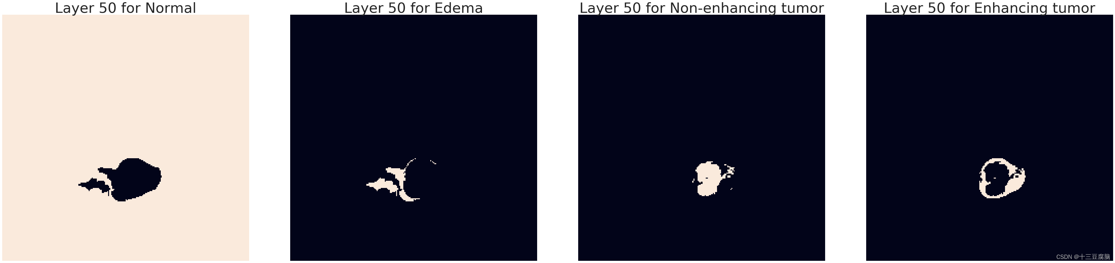

跨层交互可视化
作为查看数据的另一种方式，运行下面的代码以创建可视化，您可以在其中通过单击按钮选择特定标签并使用滑块滚动图层来选择要查看的类！

# Create button values
select_class = ToggleButtons(
    options=['Normal','Edema', 'Non-enhancing tumor', 'Enhancing tumor'],
    description='Select Class:',
    disabled=False,
    button_style='info', 
    
)
# Create layer slider
select_layer = IntSlider(min=0, max=154, description='Select Layer', continuous_update=False)

    
# Define a function for plotting images
def plot_image(seg_class, layer):
    print(f"Plotting {layer} Layer Label: {seg_class}")
    img_label = classes_dict[seg_class]
    mask = np.where(label_array[:,:,layer] == img_label, 255, 0)
    plt.figure(figsize=(10,5))
    plt.imshow(mask, cmap='gray')
    plt.axis('off');

# Use the interactive() tool to create the visualization
interactive(plot_image, seg_class=select_class, layer=select_layer)

Select Class: Normal Edema Non-enhancing tumor Enhancing tumor

Select Layer

Plotting 70 Layer Label: Enhancing tumor

二、提取一个子部分

在本周的作业中，您将提取 MRI 数据的子部分来训练您的网络。这样做的原因是，在完整的 MRI 扫描上进行训练会占用大量内存而无法实用。要在作业中提取子部分，您需要编写一个函数来隔离一小块数据以进行训练。此示例旨在向您展示如何对一维数组进行此类提取。在作业中，您将在 3D 中应用相同的逻辑。

import numpy as np
import keras
import pandas as pd

# Define a simple one dimensional "image" to extract from
image = np.array([10,11,12,13,14,15])
image

# Compute the dimensions of your "image"
image_length = image.shape[0]
image_length

array([10, 11, 12, 13, 14, 15])

1.子部分

在作业中，您将定义三个维度的“补丁大小”，这将是您要提取的子部分的大小。对于本练习，您只需要在一维中定义一个补丁大小。

要提取长度为 patch_length 的补丁，您将首先定义开始补丁的索引。运行下一个单元格以定义您的起始索引。

# Define a patch length, which will be the size of your extracted sub-section
patch_length = 3

# Define your start index
start_i = 0

在下一个单元格的末尾，您将 1 添加到起始索引。运行单元格几次以从“图像”中提取一些一维子部分

当你碰到图像的边缘时会发生什么（当 start_index 大于 3 时）？

# Define an end index given your start index and patch size
print(f"start index {start_i}")
end_i = start_i + patch_length
print(f"end index {end_i}")

# Extract a sub-section from your "image"
sub_section = image[start_i: end_i]
print("output patch length: ", len(sub_section))
print("output patch array: ", sub_section)

# Add one to your start index
start_i +=1

start index 0
end index 3
output patch length:  3
output patch array:  [10 11 12]

start index 1
end index 4
output patch length:  3
output patch array:  [11 12 13]

start index 2
end index 5
output patch length:  3
output patch array:  [12 13 14]

start index 3
end index 6
output patch length:  3
output patch array:  [13 14 15]

start index 4
end index 7
output patch length:  2
output patch array:  [14 15]

您会注意到，当您多次运行上述内容时，最终返回的子部分不再是长度 patch_length。

在作业中，您的神经网络将期望特定的子部分大小，并且不会接受其他维度的输入。对于起始索引，您将随机选择值，并且您需要确保设置随机数生成器以避免图像对象的边缘。

接下来的几个代码单元演示了如何为简单的一维示例确定起始索引的约束。

# Set your start index to 3 to extract a valid patch
start_i = 3
print(f"start index {start_i}")
end_i = start_i + patch_length
print(f"end index {end_i}")
sub_section = image[start_i: end_i]
print("output patch array: ", sub_section)

start index 3
end index 6
output patch array:  [13 14 15]

# Compute and print the largest valid value for start index
print(f"The largest start index for which "
      f"a sub section is still valid is "
      f"{image_length - patch_length}")

The largest start index for which a sub section is still valid is 3

# Compute and print the range of valid start indices
print(f"The range of valid start indices is:")

# Compute valid start indices, note the range() function excludes the upper bound
valid_start_i = [i for i in range(image_length - patch_length + 1)]
print(valid_start_i)

The range of valid start indices is:
[0, 1, 2, 3]

1.1 起始指数的随机选择

在作业中，您需要为三个维度中的每个维度中的起始索引随机选择一个有效整数。这样做的方法是按照上面的逻辑来识别有效的起始索引，然后从该有效数字范围中随机选择。

运行下一个单元格以选择一维示例的有效起始索引

# Choose a random start index, note the np.random.randint() function excludes the upper bound.
start_i = np.random.randint(image_length - patch_length + 1)
print(f"randomly selected start index {start_i}")

randomly selected start index 0

# Randomly select multiple start indices in a loop
for _ in range(10):
    start_i = np.random.randint(image_length - patch_length + 1)
    print(f"randomly selected start index {start_i}")

randomly selected start index 0
randomly selected start index 1
randomly selected start index 0
randomly selected start index 0
randomly selected start index 1
randomly selected start index 3
randomly selected start index 0
randomly selected start index 2
randomly selected start index 3
randomly selected start index 1

2. 背景比例

您将在作业中做的另一件事是计算背景与水肿和肿瘤区域的比率。您将获得一个包含以下类别标签的文件：

0：背景
1：水肿
2：非强化肿瘤
3：增强肿瘤
让我们尝试在 1-D 中演示这一点，以便在稍后的作业中获得一些关于如何在 3D 中实现它的直觉。

# We first simulate input data by defining a random patch of length 16. This will contain labels 
# with the categories (0 to 3) as defined above.

patch_labels = np.random.randint(0, 4, (16))
print(patch_labels)

[1 0 1 1 0 1 3 0 0 1 2 2 2 0 0 0]

# A straightforward approach to get the background ratio is
# to count the number of 0's and divide by the patch length

bgrd_ratio = np.count_nonzero(patch_labels == 0) / len(patch_labels)
print("using np.count_nonzero(): ", bgrd_ratio)

bgrd_ratio = len(np.where(patch_labels == 0)[0]) / len(patch_labels)
print("using np.where(): ", bgrd_ratio)

using np.count_nonzero():  0.4375
using np.where():  0.4375

# However, take note that we'll use our label array to train a neural network
# so we can opt to compute the ratio a bit later after we do some preprocessing. 
# First, we convert the label's categories into one-hot format so it can be used to train the model

patch_labels_one_hot = keras.utils.to_categorical(patch_labels, num_classes=4)
print(patch_labels_one_hot)

[[0. 1. 0. 0.]
 [1. 0. 0. 0.]
 [0. 1. 0. 0.]
 [0. 1. 0. 0.]
 [1. 0. 0. 0.]
 [0. 1. 0. 0.]
 [0. 0. 0. 1.]
 [1. 0. 0. 0.]
 [1. 0. 0. 0.]
 [0. 1. 0. 0.]
 [0. 0. 1. 0.]
 [0. 0. 1. 0.]
 [0. 0. 1. 0.]
 [1. 0. 0. 0.]
 [1. 0. 0. 0.]
 [1. 0. 0. 0.]]

注意：在上面的简单示例中，我们将类的数量硬编码为 4。在作业中，您应该考虑到标签文件可以有不同数量的类别

# Let's convert the output to a dataframe just so we can see the labels more clearly

pd.DataFrame(patch_labels_one_hot, columns=['background', 'edema', 'non-enhancing tumor', 'enhancing tumor'])

background	edema	non-enhancing tumor	enhancing tumor
0	0.0	1.0	0.0	0.0
1	1.0	0.0	0.0	0.0
2	0.0	1.0	0.0	0.0
3	0.0	1.0	0.0	0.0
4	1.0	0.0	0.0	0.0
5	0.0	1.0	0.0	0.0
6	0.0	0.0	0.0	1.0
7	1.0	0.0	0.0	0.0
8	1.0	0.0	0.0	0.0
9	0.0	1.0	0.0	0.0
10	0.0	0.0	1.0	0.0
11	0.0	0.0	1.0	0.0
12	0.0	0.0	1.0	0.0
13	1.0	0.0	0.0	0.0
14	1.0	0.0	0.0	0.0
15	1.0	0.0	0.0	0.0

# What we're interested in is the first column because that 
# indicates if the element is part of the background
# In this case, 1 = background, 0 = non-background

print("background column: ", patch_labels_one_hot[:,0])

background column:  [0. 1. 0. 0. 1. 0. 0. 1. 1. 0. 0. 0. 0. 1. 1. 1.]

# we can compute the background ratio by counting the number of 1's 
# in the said column divided by the length of the patch

bgrd_ratio = np.sum(patch_labels_one_hot[:,0])/ len(patch_labels)
print("using one-hot column: ", bgrd_ratio)

using one-hot column:  0.4375

三、U-Net模型

在本周的作业中，您将使用一种称为“U-Net”的网络架构。这种网络架构的名称来自它的 U 形形状，如图所示（图片来自维基百科上的 U-net 条目）：

U-nets 通常用于图像分割，这将是你在接下来的作业中的任务。您实际上不需要在作业中实现 U-Net，但我们希望在您在作业中使用它之前，让您有机会在此处熟悉此架构。

从图中可以看出，该架构具有一系列通过最大池化操作连接的下卷积，然后是通过上采样和连接操作连接的一系列上卷积。每个下卷积也直接连接到网络上采样部分的串联操作。有关 U-Net 架构的更多详细信息，请查看 Ronneberger 等人的原始 U-Net 论文。 2015 年。

在本实验中，您将使用 Keras 创建一个基本的 U-Net。

# Import the elements you'll need to build your U-Net
import keras
from keras import backend as K
from keras.engine import Input, Model
from keras.layers import Conv3D, MaxPooling3D, UpSampling3D, Activation, BatchNormalization, PReLU, Deconvolution3D
from keras.optimizers import Adam
from keras.layers.merge import concatenate
# Set the image shape to have the channels in the first dimension
K.set_image_data_format("channels_first")

import tensorflow as tf
tf.compat.v1.logging.set_verbosity(tf.compat.v1.logging.ERROR)

1. U-Net 的“深度”

U-Net 的“深度”等于您将使用的下卷积数。在上图中，深度为 4，因为左侧有 4 个向下卷积，包括 U 的最底部。

对于本练习，您将使用的U-Net深度为2，这意味着您的网络中将有 2 个下卷积。

1.1 输入层及其“深度”

在本实验和作业中，您将进行 3D 图像分割，也就是说，除了“高度”和“宽度”之外，您的输入层还将具有“长度”。我们在这里故意使用“长度”一词而不是“深度”来描述输入的第三空间维度，以免将其与上面定义的网络深度混淆。

输入层的形状是 (num_channels, height, width, length)，其中 num_channels 你可以把它想象成图像中的颜色通道，高度、宽度和长度只是输入的大小。

对于作业，值将是：

频道数：4
高度：160
宽度：160
长度：16

# Define an input layer tensor of the shape you'll use in the assignment
input_layer = Input(shape=(4, 160, 160, 16))
input_layer

<tf.Tensor 'input_1:0' shape=(?, 4, 160, 160, 16) dtype=float32>

请注意，张量形状有一个“？” 作为第一个维度。这将是批量（batch_size）大小。所以张量的维度是：(batch_size, num_channels, height, width, length)

2. 收缩（向下）路径

在这里，您将首先在网络中构建下行路径（U-Net 的左侧）。当您沿着这条路径移动时，输入的（高度、宽度、长度）会变小，并且通道数会增加。

2.1 深度 0

这里的“深度 0”是指 U-net 中第一个下卷积的深度。

为每个深度和该深度内的每个层指定过滤器的数量。

用于计算过滤器数量的公式是：
$filters_{i}= 32\times 2^{i}$

其中 i 是当前深度。

所以在深度 i=0 ：
过滤器0=32×(20)=32

2.2 第 0 层

每个深度有两个卷积层

# Define a Conv3D tensor with 32 filters
down_depth_0_layer_0 = Conv3D(filters=32, 
                              kernel_size=(3,3,3),
                              padding='same',
                              strides=(1,1,1)
                              )(input_layer)
down_depth_0_layer_0

<tf.Tensor 'conv3d_1/add:0' shape=(?, 32, 160, 160, 16) dtype=float32>

请注意，使用 32 个过滤器，您得到的结果是具有 32 个通道的张量。

运行下一个单元格以将 relu 激活添加到第一个卷积层

# Add a relu activation to layer 0 of depth 0
down_depth_0_layer_0 = Activation('relu')(down_depth_0_layer_0)
down_depth_0_layer_0

<tf.Tensor 'activation_1/Relu:0' shape=(?, 32, 160, 160, 16) dtype=float32>

2.3 深度 0，第 1 层

对于深度为0的第1层，滤波器个数的计算公式为：
$filters_{i}=32\times 2^{i}\times 2$

其中 i 是当前深度。

请注意，该表达式末尾的“×2”对于第 0 层不存在。
因此，对于第 1 层，在深度 i=0 处：
过滤器0=32×(1)×2=64

# Create a Conv3D layer with 64 filters and add relu activation
down_depth_0_layer_1 = Conv3D(filters=64, 
                kernel_size=(3,3,3),
                padding='same',
                strides=(1,1,1)
               )(down_depth_0_layer_0)
down_depth_0_layer_1 = Activation('relu')(down_depth_0_layer_1)
down_depth_0_layer_1

<tf.Tensor 'activation_2/Relu:0' shape=(?, 64, 160, 160, 16) dtype=float32>

2.4 最大池化

在 U-Net 架构中，每次下卷积（不包括 U 底部的最后一个下卷积）之后都有一个最大池化操作。通常，这意味着您将在每次向下卷积后添加最大池化，直至（但不包括）(深度 - 1) 次向下卷积（因为您从 0 开始计数）。

对于本实验练习：

您正在构建的 U-Net 的总深度为 2
所以你的 U 底部的深度指数为： 2−1=1 。
到目前为止，您只定义了 depth=0 下卷积，所以接下来要做的是添加最大池化
运行下一个单元以将最大池操作添加到您的 U-Net

# Define a max pooling layer
down_depth_0_layer_pool = MaxPooling3D(pool_size=(2,2,2))(down_depth_0_layer_1)
down_depth_0_layer_pool

<tf.Tensor 'max_pooling3d_1/transpose_1:0' shape=(?, 64, 80, 80, 8) dtype=float32>

2.4.1 深度 1，第 0 层
在深度 1，第 0 层，过滤器数量的计算公式为：
$filters_{i}= 32\times 2^{i}$

其中 i 是当前深度。

所以在深度 i=1 ：
过滤器1=32×(2)=64

运行下一个单元以通过激活 relu 将 Conv3D 层添加到您的网络

# Add a Conv3D layer to your network with relu activation
down_depth_1_layer_0 = Conv3D(filters=64, 
                kernel_size=(3,3,3),
                padding='same',
                strides=(1,1,1)
               )(down_depth_0_layer_pool)
down_depth_1_layer_0 = Activation('relu')(down_depth_1_layer_0)
down_depth_1_layer_0

<tf.Tensor 'activation_3/Relu:0' shape=(?, 64, 80, 80, 8) dtype=float32>

2.4.2 深度 1，第 1 层
对于深度 1 的第 1 层，您将用于过滤器数量的公式是：
$filters_{i}=32\times 2^{i}\times 2$

其中 i 是当前深度。

请注意，此表达式末尾的“×2”不存在于第 0 层。
所以在深度 i=1 ：
过滤器1=32×(2)×2=128

运行下一个单元以将具有 128 个过滤器的另一个 Conv3D 添加到您的网络。

# Add another Conv3D with 128 filters to your network.
down_depth_1_layer_1 = Conv3D(filters=128, 
                kernel_size=(3,3,3),
                padding='same',
                strides=(1,1,1)
               )(down_depth_1_layer_0)
down_depth_1_layer_1 = Activation('relu')(down_depth_1_layer_1)
down_depth_1_layer_1

<tf.Tensor 'activation_4/Relu:0' shape=(?, 128, 80, 80, 8) dtype=float32>

在深度 1（U 的底部）没有最大池化
当你到达 U-net 的“底部”时，你不需要在卷积之后应用最大池化。

3. 扩展（向上）路径

现在您将处理 U-Net 的扩展路径（查看图表时在右侧向上）。图像的（高度、宽度、长度）都在扩展路径中变大。

3.1 深度0，上采样层0

您将使用 (2,2,2) 的池大小进行上采样。

这是 tf.keras.layers.UpSampling3D 的默认值
作为深度 1 的上采样的输入，您将使用下采样的最后一层。在这种情况下，它是深度 1 层 1。
运行下一个单元以向您的网络添加上采样操作。请注意，您没有向此上采样层添加任何激活。

# Add an upsampling operation to your network
up_depth_0_layer_0 = UpSampling3D(size=(2,2,2))(down_depth_1_layer_1)
up_depth_0_layer_0

<tf.Tensor 'up_sampling3d_1/concat_2:0' shape=(?, 128, 160, 160, 16) dtype=float32>

3.2 连接上采样深度 0 和下采样深度 0

现在，您将使用深度为 0 的图层应用串联操作。

up_depth_0_layer_0：形状为 (?, 128, 160, 160, 16)
depth_0_layer_1：形状为 (?, 64, 160, 160, 16)

仔细检查这两层是否具有相同的高度、宽度和长度。

如果它们相同，则可以沿轴 1（通道轴）连接它们。
两者的 (height, width, length) 都是 (160, 160, 16)。
运行下一个单元格以检查您要连接的图层是否具有相同的高度、宽度和长度。

# Print the shape of layers to concatenate
print(up_depth_0_layer_0)
print()
print(down_depth_0_layer_1)

Tensor("up_sampling3d_1/concat_2:0", shape=(?, 128, 160, 160, 16), dtype=float32)

Tensor("activation_2/Relu:0", shape=(?, 64, 160, 160, 16), dtype=float32)

运行下一个单元以将串联操作添加到您的网络

# Add a concatenation along axis 1
up_depth_1_concat = concatenate([up_depth_0_layer_0,
                                 down_depth_0_layer_1],
                                axis=1)
up_depth_1_concat

<tf.Tensor 'concatenate_1/concat:0' shape=(?, 192, 160, 160, 16) dtype=float32>

请注意，上采样层有 128 个通道，下卷积层有 64 个通道，因此当连接时，结果有 128 + 64 = 192 个通道。

3.3 上卷积第 1 层

该层的过滤器数量将设置为下卷积层 1 中相同深度 0 (down_depth_0_layer_1) 的通道数。

运行下一个单元格看看下卷积深度0第1层的形状

down_depth_0_layer_1

<tf.Tensor 'activation_2/Relu:0' shape=(?, 64, 160, 160, 16) dtype=float32>

注意 depth_0_layer_1 的通道数是 64

print(f"number of filters: {down_depth_0_layer_1._keras_shape[1]}")

# Add a Conv3D up-convolution with 64 filters to your network
up_depth_1_layer_1 = Conv3D(filters=64, 
                            kernel_size=(3,3,3),
                            padding='same',
                            strides=(1,1,1)
                           )(up_depth_1_concat)
up_depth_1_layer_1 = Activation('relu')(up_depth_1_layer_1)
up_depth_1_layer_1

number of filters: 64

<tf.Tensor 'activation_5/Relu:0' shape=(?, 64, 160, 160, 16) dtype=float32>

3.4 上卷积深度0，第2层

在上卷积中深度为 0 的第 2 层，下一步将是添加另一个上卷积。您要用于下一次上卷积的过滤器数量需要等于下卷积深度 0 层 1 中的过滤器数量。

运行下一个单元格以提醒自己下卷积深度 0 层 1 中的过滤器数量。

print(down_depth_0_layer_1)
print(f"number of filters: {down_depth_0_layer_1._keras_shape[1]}")

Tensor("activation_2/Relu:0", shape=(?, 64, 160, 160, 16), dtype=float32)
number of filters: 64

如您所见，down_depth_0_layer_1 中的通道/过滤器数量为 64。

运行下一个单元格以将具有 64 个过滤器的 Conv3D 上卷积添加到您的网络。

# Add a Conv3D up-convolution with 64 filters to your network
up_depth_1_layer_2 = Conv3D(filters=64, 
                            kernel_size=(3,3,3),
                            padding='same',
                            strides=(1,1,1)
                           )(up_depth_1_layer_1)
up_depth_1_layer_2 = Activation('relu')(up_depth_1_layer_2)
up_depth_1_layer_2

<tf.Tensor 'activation_6/Relu:0' shape=(?, 64, 160, 160, 16) dtype=float32>

4. 最终卷积

对于最终卷积，您将设置过滤器的数量等于输入数据中的类数。

在作业中，您将使用 3 个类的数据，即：

1：水肿
2：非强化肿瘤
3：增强肿瘤
运行下一个单元以将具有 3 个过滤器的最终 Conv3D 添加到您的网络。

# Add a final Conv3D with 3 filters to your network.
final_conv = Conv3D(filters=3, #3 categories 
                    kernel_size=(1,1,1),
                    padding='valid',
                    strides=(1,1,1)
                    )(up_depth_1_layer_2)
final_conv

<tf.Tensor 'conv3d_7/add:0' shape=(?, 3, 160, 160, 16) dtype=float32>

4.1 最终卷积的激活

运行下一个单元格以将 sigmoid 激活添加到您的最终卷积中。

# Add a sigmoid activation to your final convolution.
final_activation = Activation('sigmoid')(final_conv)
final_activation

<tf.Tensor 'activation_7/Sigmoid:0' shape=(?, 3, 160, 160, 16) dtype=float32>

4.2 创建和编译模型

在此示例中，您将设置损失和指标为 Keras 中预建的选项。但是，在作业中，您将实现更好的损失函数和指标来评估模型的性能。

运行下一个单元以根据您在上面创建的架构定义和编译模型。

# Define and compile your model
model = Model(inputs=input_layer, outputs=final_activation)
model.compile(optimizer=Adam(lr=0.00001),
              loss='categorical_crossentropy',
              metrics=['categorical_accuracy']
             )


# Print out a summary of the model you created
model.summary()

Model: "model_1"
__________________________________________________________________________________________________
Layer (type)                    Output Shape         Param #     Connected to                     
==================================================================================================
input_1 (InputLayer)            (None, 4, 160, 160,  0                                            
__________________________________________________________________________________________________
conv3d_1 (Conv3D)               (None, 32, 160, 160, 3488        input_1[0][0]                    
__________________________________________________________________________________________________
activation_1 (Activation)       (None, 32, 160, 160, 0           conv3d_1[0][0]                   
__________________________________________________________________________________________________
conv3d_2 (Conv3D)               (None, 64, 160, 160, 55360       activation_1[0][0]               
__________________________________________________________________________________________________
activation_2 (Activation)       (None, 64, 160, 160, 0           conv3d_2[0][0]                   
__________________________________________________________________________________________________
max_pooling3d_1 (MaxPooling3D)  (None, 64, 80, 80, 8 0           activation_2[0][0]               
__________________________________________________________________________________________________
conv3d_3 (Conv3D)               (None, 64, 80, 80, 8 110656      max_pooling3d_1[0][0]            
__________________________________________________________________________________________________
activation_3 (Activation)       (None, 64, 80, 80, 8 0           conv3d_3[0][0]                   
__________________________________________________________________________________________________
conv3d_4 (Conv3D)               (None, 128, 80, 80,  221312      activation_3[0][0]               
__________________________________________________________________________________________________
activation_4 (Activation)       (None, 128, 80, 80,  0           conv3d_4[0][0]                   
__________________________________________________________________________________________________
up_sampling3d_1 (UpSampling3D)  (None, 128, 160, 160 0           activation_4[0][0]               
__________________________________________________________________________________________________
concatenate_1 (Concatenate)     (None, 192, 160, 160 0           up_sampling3d_1[0][0]            
                                                                 activation_2[0][0]               
__________________________________________________________________________________________________
conv3d_5 (Conv3D)               (None, 64, 160, 160, 331840      concatenate_1[0][0]              
__________________________________________________________________________________________________
activation_5 (Activation)       (None, 64, 160, 160, 0           conv3d_5[0][0]                   
__________________________________________________________________________________________________
conv3d_6 (Conv3D)               (None, 64, 160, 160, 110656      activation_5[0][0]               
__________________________________________________________________________________________________
activation_6 (Activation)       (None, 64, 160, 160, 0           conv3d_6[0][0]                   
__________________________________________________________________________________________________
conv3d_7 (Conv3D)               (None, 3, 160, 160,  195         activation_6[0][0]               
__________________________________________________________________________________________________
activation_7 (Activation)       (None, 3, 160, 160,  0           conv3d_7[0][0]                   
==================================================================================================
Total params: 833,507
Trainable params: 833,507
Non-trainable params: 0
__________________________________________________________________________________________________

恭喜！您已经创建了自己的 U-Net 模型架构！
接下来，您将通过将模型摘要与下面定义的示例模型进行比较来检查您是否正确执行了所有操作。

4.2.1 仔细检查你的模型
要仔细检查您是否创建了正确的模型，请使用我们提供的函数来创建相同的模型，并检查图层和图层尺寸是否匹配！

# Import predefined utilities
import util

# Create a model using a predefined function
model_2 = util.unet_model_3d(depth=2,
                                loss_function='categorical_crossentropy',
                                metrics=['categorical_accuracy'])

# Print out a summary of the model created by the predefined function
model_2.summary()

Model: "model_2"
__________________________________________________________________________________________________
Layer (type)                    Output Shape         Param #     Connected to                     
==================================================================================================
input_2 (InputLayer)            (None, 4, 160, 160,  0                                            
__________________________________________________________________________________________________
conv3d_8 (Conv3D)               (None, 32, 160, 160, 3488        input_2[0][0]                    
__________________________________________________________________________________________________
activation_8 (Activation)       (None, 32, 160, 160, 0           conv3d_8[0][0]                   
__________________________________________________________________________________________________
conv3d_9 (Conv3D)               (None, 64, 160, 160, 55360       activation_8[0][0]               
__________________________________________________________________________________________________
activation_9 (Activation)       (None, 64, 160, 160, 0           conv3d_9[0][0]                   
__________________________________________________________________________________________________
max_pooling3d_2 (MaxPooling3D)  (None, 64, 80, 80, 8 0           activation_9[0][0]               
__________________________________________________________________________________________________
conv3d_10 (Conv3D)              (None, 64, 80, 80, 8 110656      max_pooling3d_2[0][0]            
__________________________________________________________________________________________________
activation_10 (Activation)      (None, 64, 80, 80, 8 0           conv3d_10[0][0]                  
__________________________________________________________________________________________________
conv3d_11 (Conv3D)              (None, 128, 80, 80,  221312      activation_10[0][0]              
__________________________________________________________________________________________________
activation_11 (Activation)      (None, 128, 80, 80,  0           conv3d_11[0][0]                  
__________________________________________________________________________________________________
up_sampling3d_2 (UpSampling3D)  (None, 128, 160, 160 0           activation_11[0][0]              
__________________________________________________________________________________________________
concatenate_2 (Concatenate)     (None, 192, 160, 160 0           up_sampling3d_2[0][0]            
                                                                 activation_9[0][0]               
__________________________________________________________________________________________________
conv3d_12 (Conv3D)              (None, 64, 160, 160, 331840      concatenate_2[0][0]              
__________________________________________________________________________________________________
activation_12 (Activation)      (None, 64, 160, 160, 0           conv3d_12[0][0]                  
__________________________________________________________________________________________________
conv3d_13 (Conv3D)              (None, 64, 160, 160, 110656      activation_12[0][0]              
__________________________________________________________________________________________________
activation_13 (Activation)      (None, 64, 160, 160, 0           conv3d_13[0][0]                  
__________________________________________________________________________________________________
conv3d_14 (Conv3D)              (None, 3, 160, 160,  195         activation_13[0][0]              
__________________________________________________________________________________________________
activation_14 (Activation)      (None, 3, 160, 160,  0           conv3d_14[0][0]                  
==================================================================================================
Total params: 833,507
Trainable params: 833,507
Non-trainable params: 0
__________________________________________________________________________________________________

查看您创建的 U-Net 的模型摘要，并将其与您在上面导入的预定义函数创建的示例模型的摘要进行比较。
这就是本练习的内容，我们希望这能让您更深入地了解您将在本周的作业中使用的网络架构！

总结

实验部分