小白学Pytorch系列--Torch API (10)

发呆的比目鱼

已于 2023-03-20 00:14:49 修改

阅读量604

点赞数

分类专栏： PyTorch框架文章标签： pytorch 深度学习人工智能

于 2023-03-19 10:42:07 首次发布

本文链接：https://blog.csdn.net/weixin_42486623/article/details/129635583

版权

PyTorch框架专栏收录该内容

52 篇文章 8 订阅

订阅专栏

小白学Pytorch系列–Torch API (10)

BLAS and LAPACK Operations

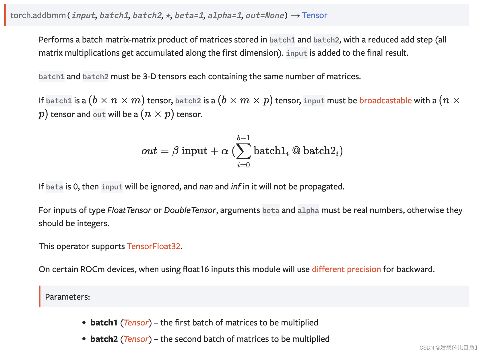
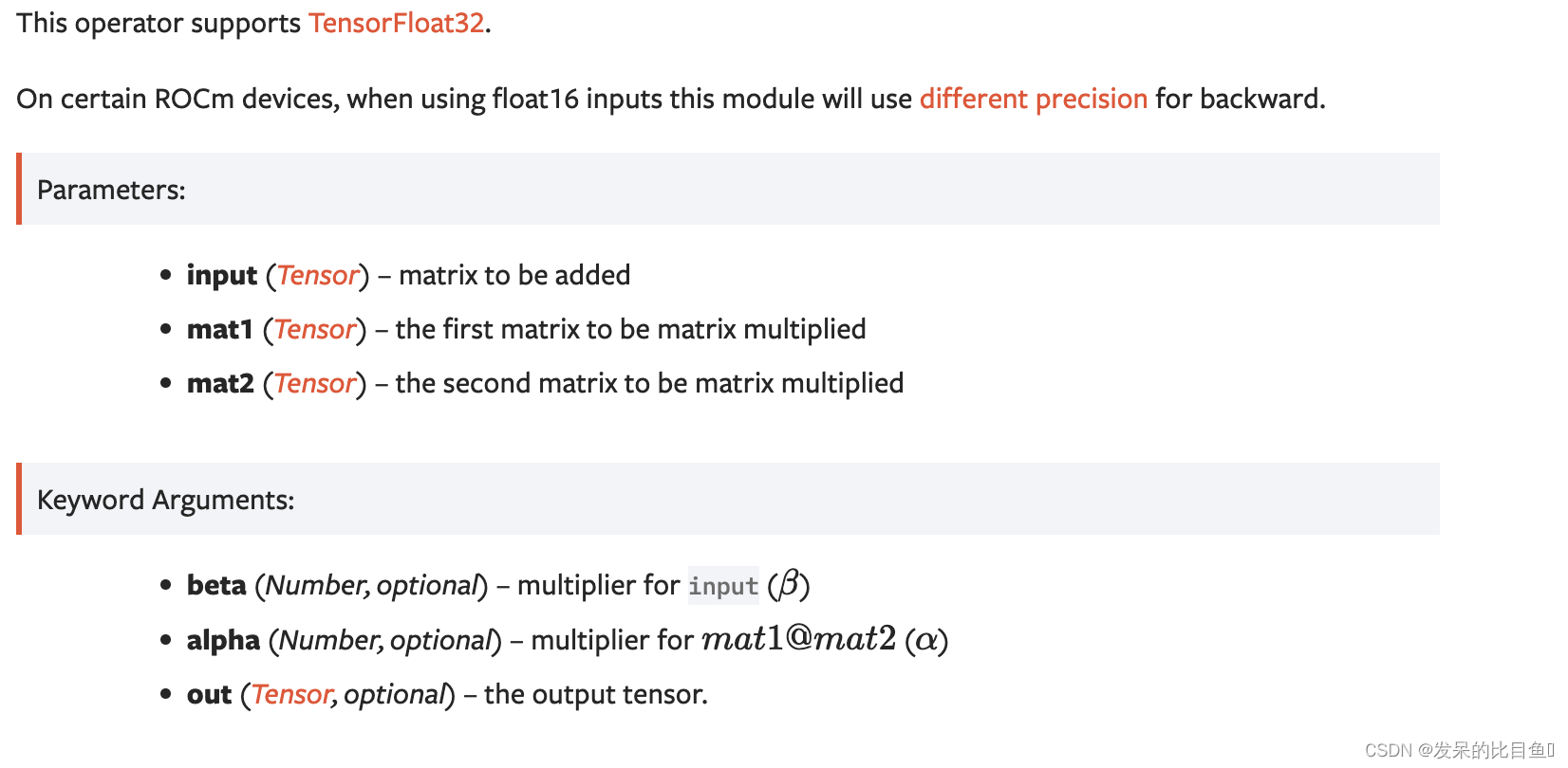
addbmm

执行存储在batch1和batch2中的矩阵的批处理矩阵矩阵乘积，并减少加法步骤（所有矩阵乘法都沿第一维累加）。将输入添加到最终结果中。

>>> M = torch.randn(3, 5)
>>> batch1 = torch.randn(10, 3, 4)
>>> batch2 = torch.randn(10, 4, 5)
>>> torch.addbmm(M, batch1, batch2)
tensor([[  6.6311,   0.0503,   6.9768, -12.0362,  -2.1653],
        [ -4.8185,  -1.4255,  -6.6760,   8.9453,   2.5743],
        [ -3.8202,   4.3691,   1.0943,  -1.1109,   5.4730]])

addmm

对矩阵mat1和mat2执行矩阵乘法运算。矩阵输入被添加到最终结果中。

>>> M = torch.randn(2, 3)
>>> mat1 = torch.randn(2, 3)
>>> mat2 = torch.randn(3, 3)
>>> torch.addmm(M, mat1, mat2)
tensor([[-4.8716,  1.4671, -1.3746],
        [ 0.7573, -3.9555, -2.8681]])

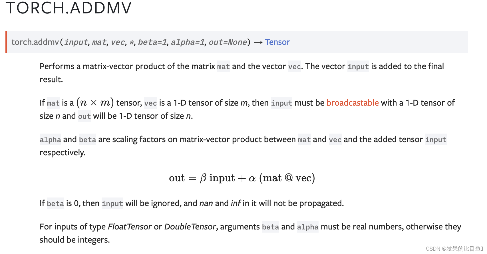
addmv

执行矩阵矩阵和向量vec的矩阵向量乘积。将矢量输入添加到最终结果中

>>> M = torch.randn(2)
>>> mat = torch.randn(2, 3)
>>> vec = torch.randn(3)
>>> torch.addmv(M, mat, vec)
tensor([-0.3768, -5.5565])

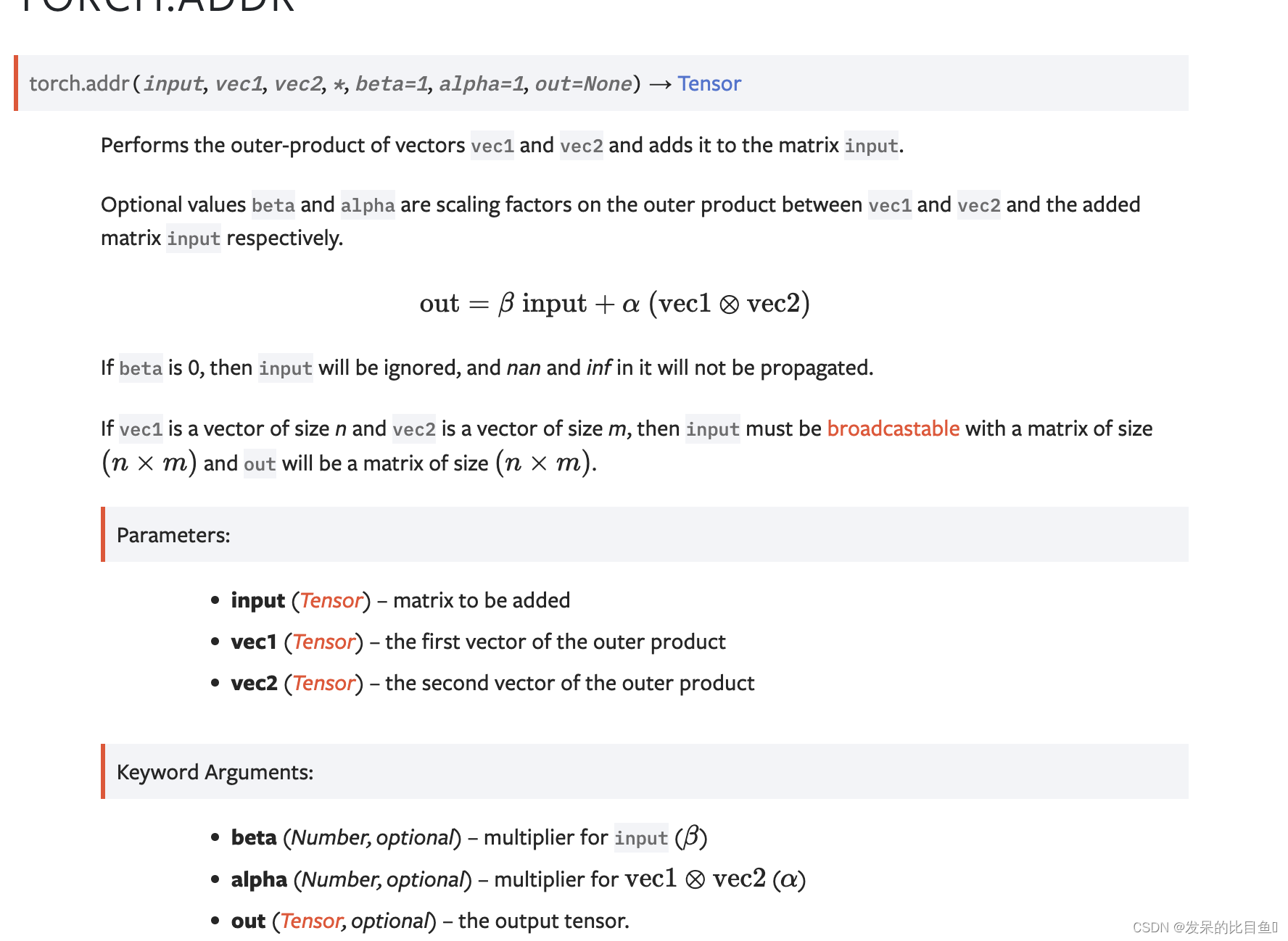
addr

执行向量vec1和vec2的外积，并将其添加到矩阵输入。

>>> vec1 = torch.arange(1., 4.)
>>> vec2 = torch.arange(1., 3.)
>>> M = torch.zeros(3, 2)
>>> torch.addr(M, vec1, vec2)
tensor([[ 1.,  2.],
        [ 2.,  4.],
        [ 3.,  6.]])

baddbmm

执行批次1和批次2中矩阵的批次矩阵矩阵乘积。将输入添加到最终结果中。

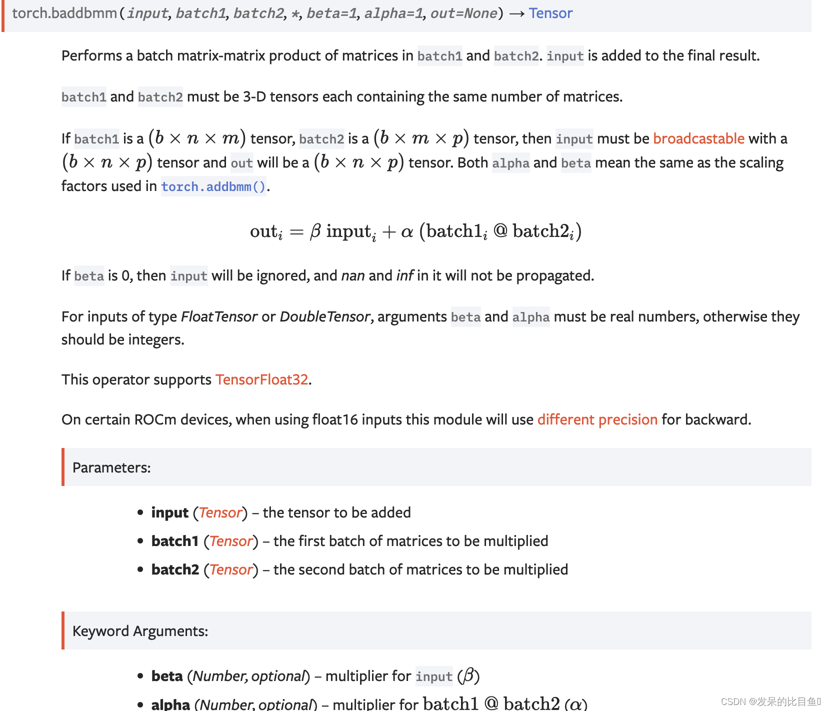
>>> M = torch.randn(10, 3, 5)
>>> batch1 = torch.randn(10, 3, 4)
>>> batch2 = torch.randn(10, 4, 5)
>>> torch.baddbmm(M, batch1, batch2).size()
torch.Size([10, 3, 5])

bmm

执行存储在input和mat2中的矩阵的批处理矩阵矩阵乘积。

input和mat2必须是3-D张量，每个张量都包含相同数量的矩阵。

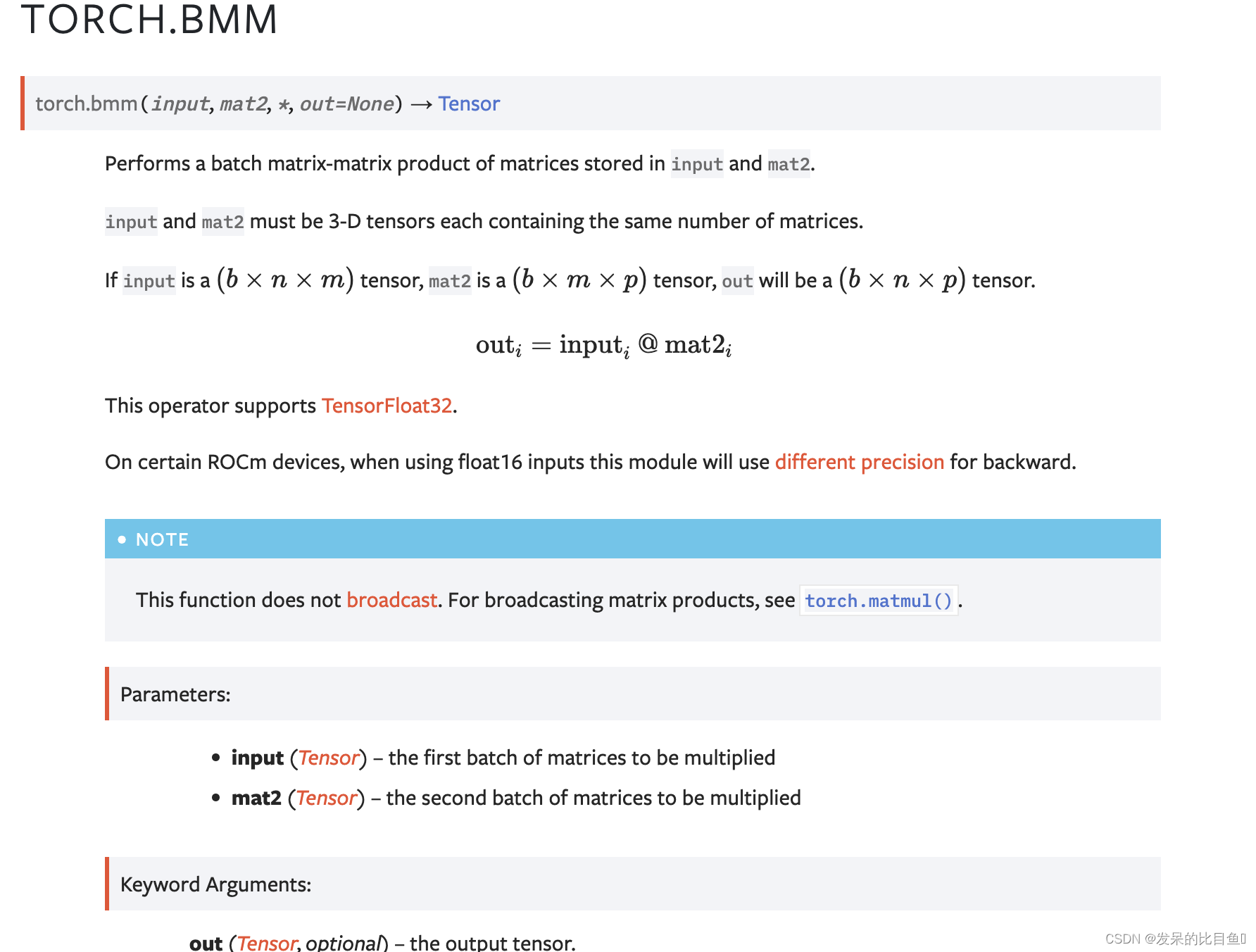
>>> input = torch.randn(10, 3, 4)
>>> mat2 = torch.randn(10, 4, 5)
>>> res = torch.bmm(input, mat2)
>>> res.size()
torch.Size([10, 3, 5])

chain_matmul

返回N个二维张量的矩阵乘积。该乘积是使用矩阵链顺序算法有效计算的，该算法选择在算术运算（[CLRS]）方面产生最低成本的顺序。注意，由于这是一个计算乘积的函数，因此N需要大于或等于2；如果等于2，则返回平凡矩阵矩阵乘积。如果N是1，那么这是一个无运算-原始矩阵按原样返回。

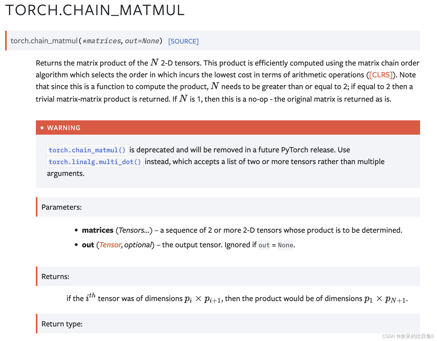
>>> a = torch.randn(3, 4)
>>> b = torch.randn(4, 5)
>>> c = torch.randn(5, 6)
>>> d = torch.randn(6, 7)
>>> # will raise a deprecation warning
>>> torch.chain_matmul(a, b, c, d)
tensor([[ -2.3375,  -3.9790,  -4.1119,  -6.6577,   9.5609, -11.5095,  -3.2614],
        [ 21.4038,   3.3378,  -8.4982,  -5.2457, -10.2561,  -2.4684,   2.7163],
        [ -0.9647,  -5.8917,  -2.3213,  -5.2284,  12.8615, -12.2816,  -2.5095]])

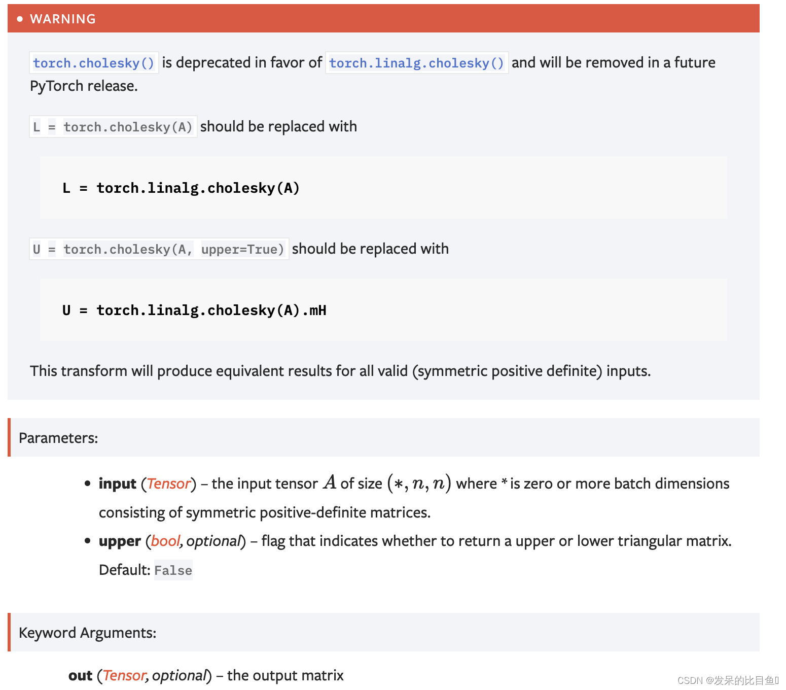
cholesky

计算对称正定矩阵A或一批对称正定矩阵的Cholesky分解。

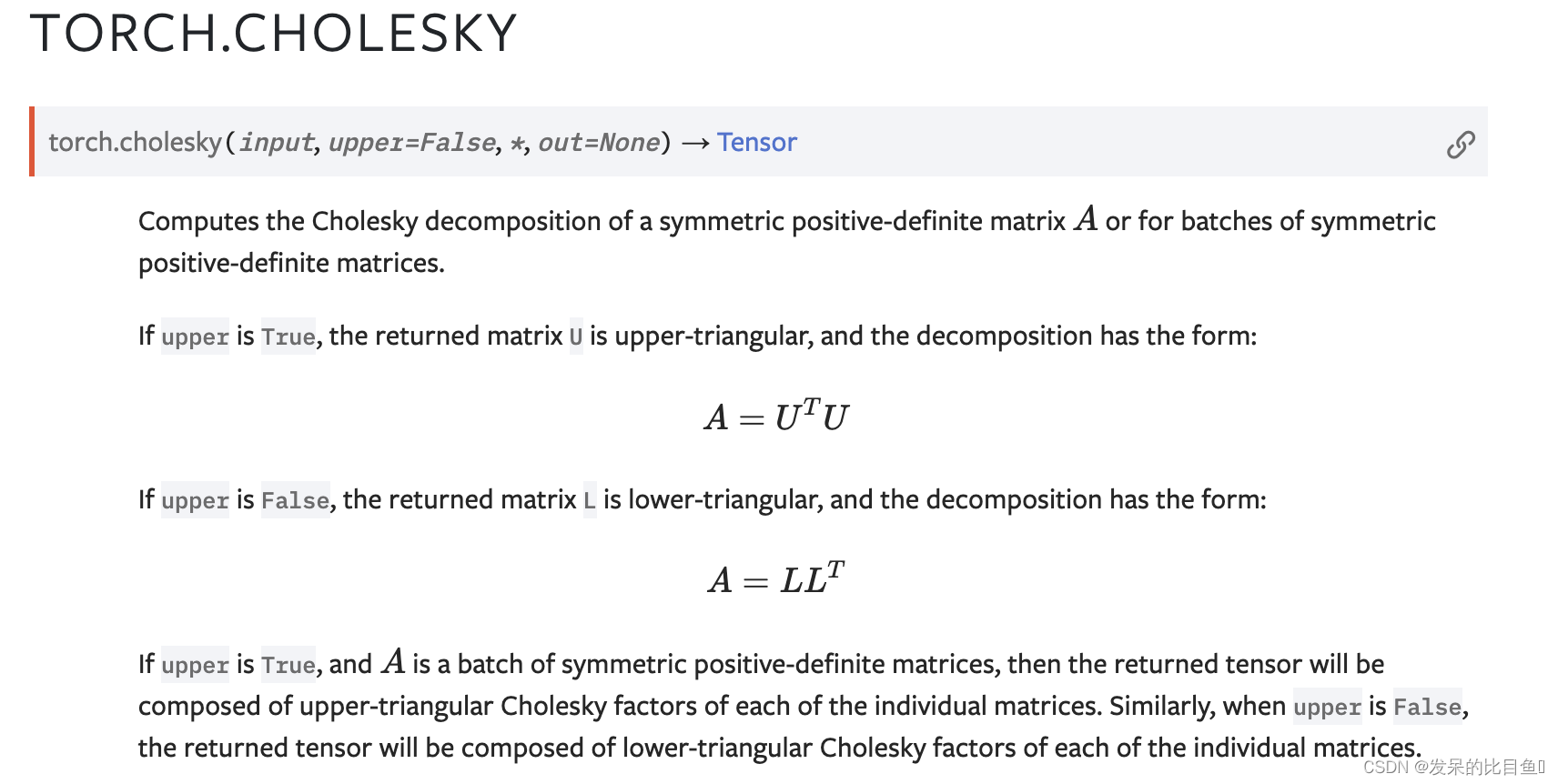
功能：
计算对称正定矩阵的Cholesky分解。A 或对于成批的对称正定矩阵。
如果 upper 为 True ，则返回的矩阵 U 为上三角，分解形式为：
$A=U^TU$
如果 upper 为 False ，则返回的矩阵 L 为下三角，分解形式为：
$A=LL^T$
如果 upper 为 True ，并且A 是一组对称的正定矩阵，则返回的张量将由各个矩阵的上三角Cholesky因子组成。同样，当 upper 为 False 时，返回的张量将由各个矩阵的下三角Cholesky因子组成。
注意：
torch.linalg.cholesky() 如果可能，应该在 torch.cholesky 上使用torch.linalg.cholesky()。但是请注意， torch.linalg.cholesky() 尚不支持 upper 参数，而是始终返回下三角矩阵。
Parameters
input（张量）–输入张量A 大小(*, n, n) 其中 * 是零个或多个由对称正定矩阵组成的批处理维。
upper（bool ，可选）–指示是否返回上三角矩阵或下三角矩阵的标志。默认值： False
输出：
out（Tensor ，可选）–输出矩阵

>>> a = torch.randn(3, 3)
>>> a = a @ a.mT + 1e-3 # make symmetric positive-definite 使对称正定
>>> l = torch.cholesky(a)
>>> a
tensor([[ 2.4112, -0.7486,  1.4551],
        [-0.7486,  1.3544,  0.1294],
        [ 1.4551,  0.1294,  1.6724]])
>>> l
tensor([[ 1.5528,  0.0000,  0.0000],
        [-0.4821,  1.0592,  0.0000],
        [ 0.9371,  0.5487,  0.7023]])
>>> l @ l.mT
tensor([[ 2.4112, -0.7486,  1.4551],
        [-0.7486,  1.3544,  0.1294],
        [ 1.4551,  0.1294,  1.6724]])
>>> a = torch.randn(3, 2, 2) # Example for batched input
>>> a = a @ a.mT + 1e-03 # make symmetric positive-definite
>>> l = torch.cholesky(a)
>>> z = l @ l.mT
>>> torch.dist(z, a)
tensor(2.3842e-07)

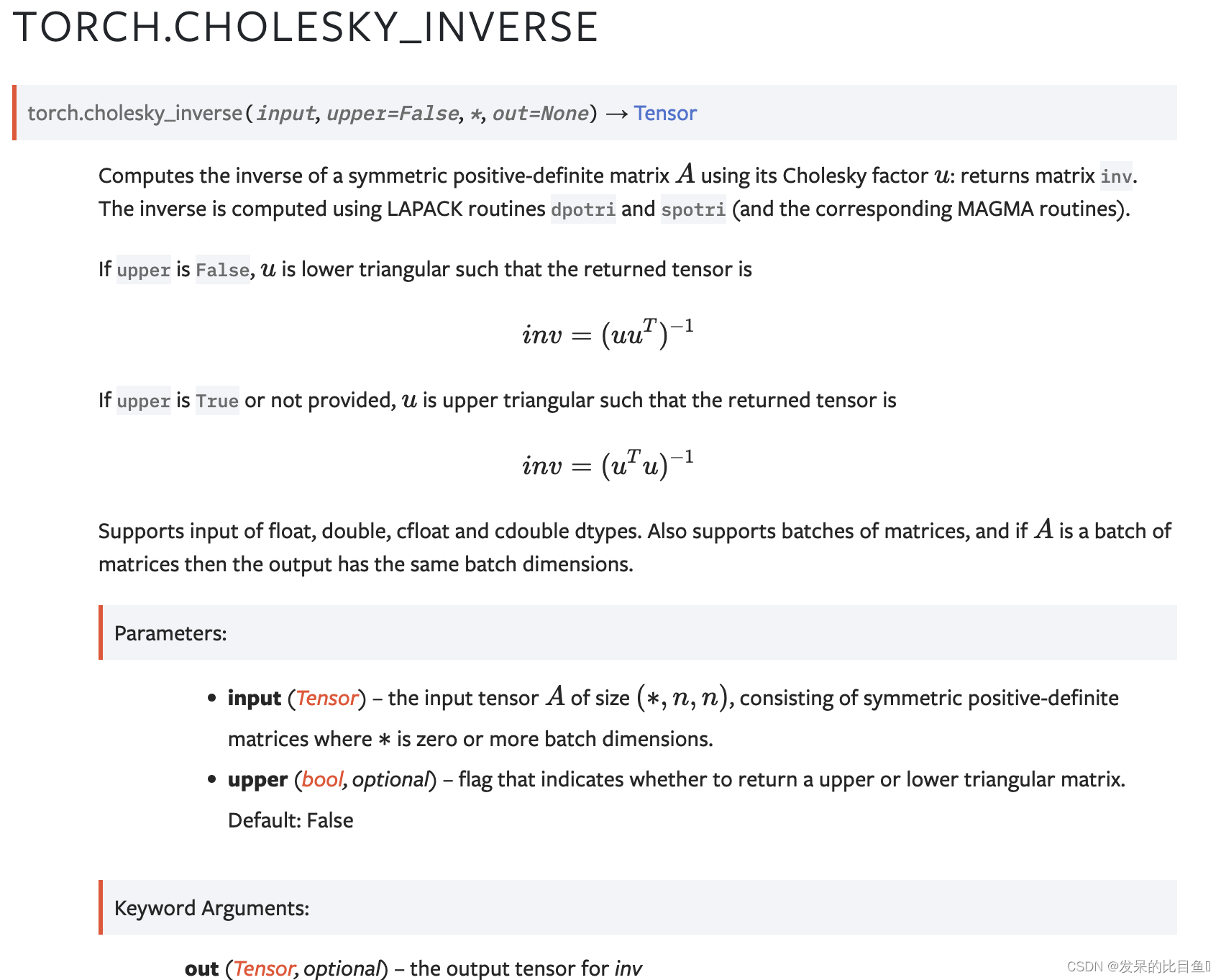
cholesky_inverse

使用Cholesky因子U计算对称正定矩阵A的逆：返回矩阵inv。逆是使用LAPACK例程dpotri和spotri（以及相应的MAGMA例程）计算的。

>>> a = torch.randn(3, 3)
>>> a = torch.mm(a, a.t()) + 1e-05 * torch.eye(3) # make symmetric positive definite
>>> u = torch.linalg.cholesky(a)
>>> a
tensor([[  0.9935,  -0.6353,   1.5806],
        [ -0.6353,   0.8769,  -1.7183],
        [  1.5806,  -1.7183,  10.6618]])
>>> torch.cholesky_inverse(u)
tensor([[ 1.9314,  1.2251, -0.0889],
        [ 1.2251,  2.4439,  0.2122],
        [-0.0889,  0.2122,  0.1412]])
>>> a.inverse()
tensor([[ 1.9314,  1.2251, -0.0889],
        [ 1.2251,  2.4439,  0.2122],
        [-0.0889,  0.2122,  0.1412]])
>>> a = torch.randn(3, 2, 2) # Example for batched input
>>> a = a @ a.mT + 1e-03 # make symmetric positive-definite
>>> l = torch.linalg.cholesky(a)
>>> z = l @ l.mT
>>> torch.dist(z, a)
tensor(3.5894e-07)

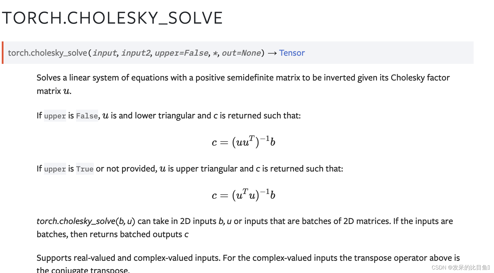
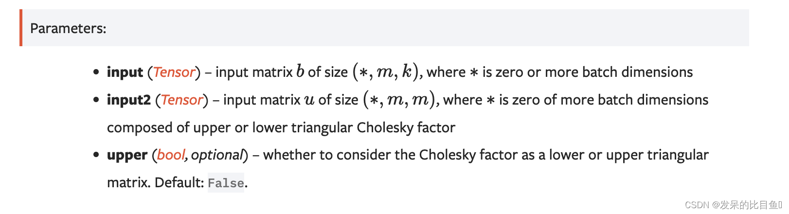
cholesky_solve

求解一个线性方程组，该方程组具有一个半正定矩阵，给定其Cholesky因子矩阵u。

>>> a = torch.randn(3, 3)
>>> a = torch.mm(a, a.t()) # make symmetric positive definite
>>> u = torch.linalg.cholesky(a)
>>> a
tensor([[ 0.7747, -1.9549,  1.3086],
        [-1.9549,  6.7546, -5.4114],
        [ 1.3086, -5.4114,  4.8733]])
>>> b = torch.randn(3, 2)
>>> b
tensor([[-0.6355,  0.9891],
        [ 0.1974,  1.4706],
        [-0.4115, -0.6225]])
>>> torch.cholesky_solve(b, u)
tensor([[ -8.1625,  19.6097],
        [ -5.8398,  14.2387],
        [ -4.3771,  10.4173]])
>>> torch.mm(a.inverse(), b)
tensor([[ -8.1626,  19.6097],
        [ -5.8398,  14.2387],
        [ -4.3771,  10.4173]])

dot

计算两个一维张量的点积。

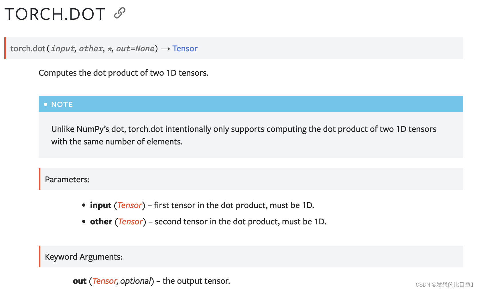
>>> torch.dot(torch.tensor([2, 3]), torch.tensor([2, 1]))
tensor(7)

geqrf

这是一个用于直接调用LAPACK的geqrf的低级函数。此函数返回geqrf的LAPACK文档中定义的命名元组(a，tau)。

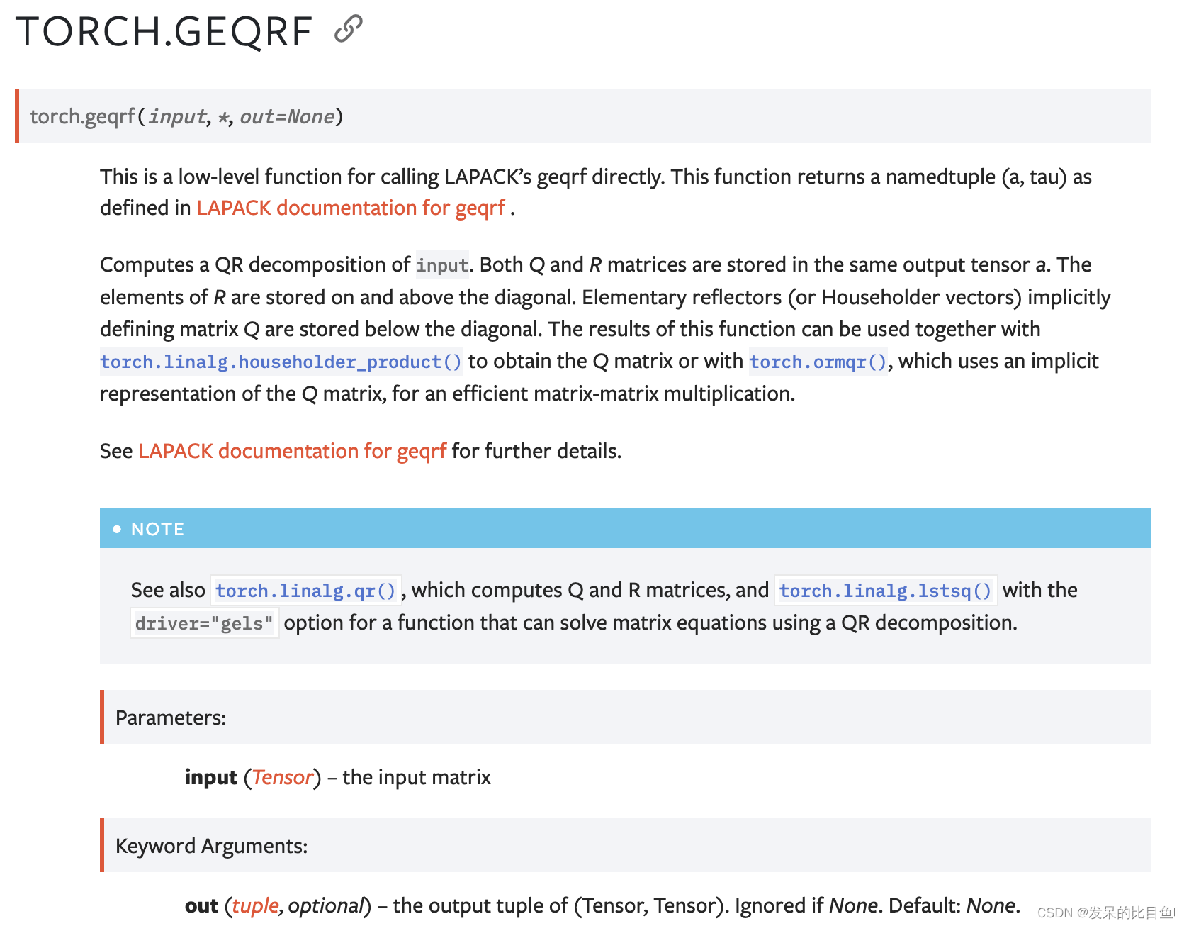
mat1 = torch.randn(10, 10)
q, r = torch.qr(mat1)
m, tau = torch.geqrf(mat1)

ger

torch.outer()的别名。

>>> v1 = torch.arange(1., 5.)
>>> v2 = torch.arange(1., 4.)
>>> torch.outer(v1, v2)
tensor([[  1.,   2.,   3.],
        [  2.,   4.,   6.],
        [  3.,   6.,   9.],
        [  4.,   8.,  12.]])

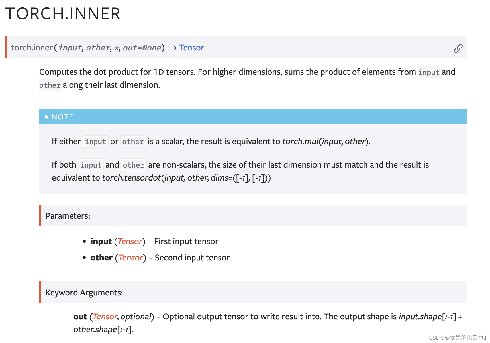
inner

计算1D张量的点积。对于较高的维度，求输入元素和其他元素沿其最后一个维度的乘积。

# Dot product
>>> torch.inner(torch.tensor([1, 2, 3]), torch.tensor([0, 2, 1]))
tensor(7)

# Multidimensional input tensors
>>> a = torch.randn(2, 3)
>>> a
tensor([[0.8173, 1.0874, 1.1784],
        [0.3279, 0.1234, 2.7894]])
>>> b = torch.randn(2, 4, 3)
>>> b
tensor([[[-0.4682, -0.7159,  0.1506],
        [ 0.4034, -0.3657,  1.0387],
        [ 0.9892, -0.6684,  0.1774],
        [ 0.9482,  1.3261,  0.3917]],

        [[ 0.4537,  0.7493,  1.1724],
        [ 0.2291,  0.5749, -0.2267],
        [-0.7920,  0.3607, -0.3701],
        [ 1.3666, -0.5850, -1.7242]]])
>>> torch.inner(a, b)
tensor([[[-0.9837,  1.1560,  0.2907,  2.6785],
        [ 2.5671,  0.5452, -0.6912, -1.5509]],

        [[ 0.1782,  2.9843,  0.7366,  1.5672],
        [ 3.5115, -0.4864, -1.2476, -4.4337]]])

# Scalar input
>>> torch.inner(a, torch.tensor(2))
tensor([[1.6347, 2.1748, 2.3567],
        [0.6558, 0.2469, 5.5787]])

inverse

计算平方矩阵的逆矩阵（如果存在）。如果矩阵不可逆，则引发RuntimeError。

>>> A = torch.randn(4, 4)
>>> Ainv = torch.linalg.inv(A)
>>> torch.dist(A @ Ainv, torch.eye(4))
tensor(1.1921e-07)

>>> A = torch.randn(2, 3, 4, 4)  # Batch of matrices
>>> Ainv = torch.linalg.inv(A)
>>> torch.dist(A @ Ainv, torch.eye(4))
tensor(1.9073e-06)

>>> A = torch.randn(4, 4, dtype=torch.complex128)  # Complex matrix
>>> Ainv = torch.linalg.inv(A)
>>> torch.dist(A @ Ainv, torch.eye(4))
tensor(7.5107e-16, dtype=torch.float64)

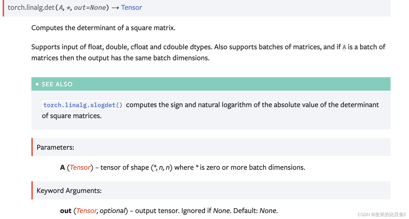
det

计算一个平方矩阵的行列式。

支持float、double、cfloat和cddouble数据类型的输入。还支持批量矩阵，如果A是一批矩阵，则输出具有相同的批量维度。

>>> A = torch.randn(3, 3)
>>> torch.linalg.det(A)
tensor(0.0934)

>>> A = torch.randn(3, 2, 2)
>>> torch.linalg.det(A)
tensor([1.1990, 0.4099, 0.7386])

logdet

计算一个正方形矩阵或一批正方形矩阵的对数行列式。

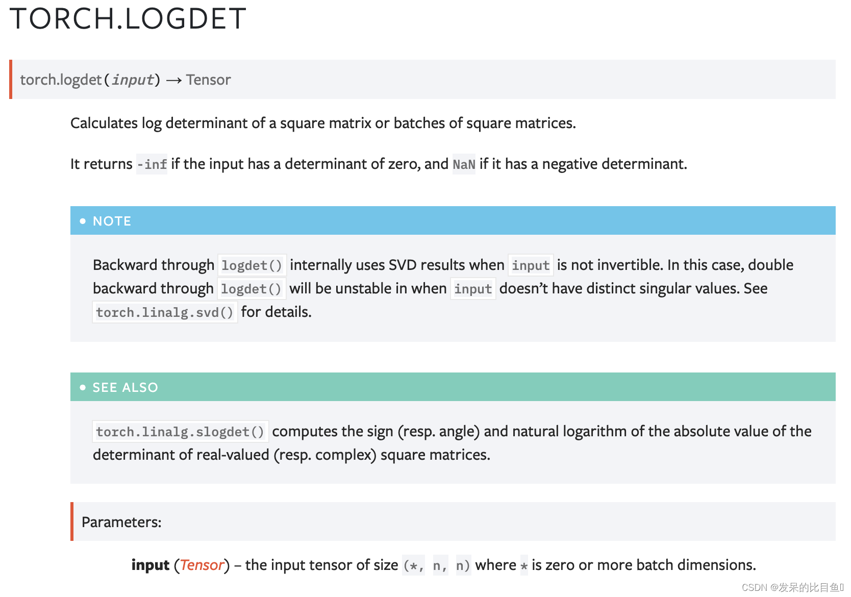
>>> A = torch.randn(3, 3)
>>> torch.det(A)
tensor(0.2611)
>>> torch.logdet(A)
tensor(-1.3430)
>>> A
tensor([[[ 0.9254, -0.6213],
         [-0.5787,  1.6843]],

        [[ 0.3242, -0.9665],
         [ 0.4539, -0.0887]],

        [[ 1.1336, -0.4025],
         [-0.7089,  0.9032]]])
>>> A.det()
tensor([1.1990, 0.4099, 0.7386])
>>> A.det().log()
tensor([ 0.1815, -0.8917, -0.3031])

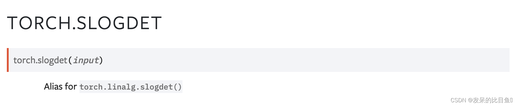
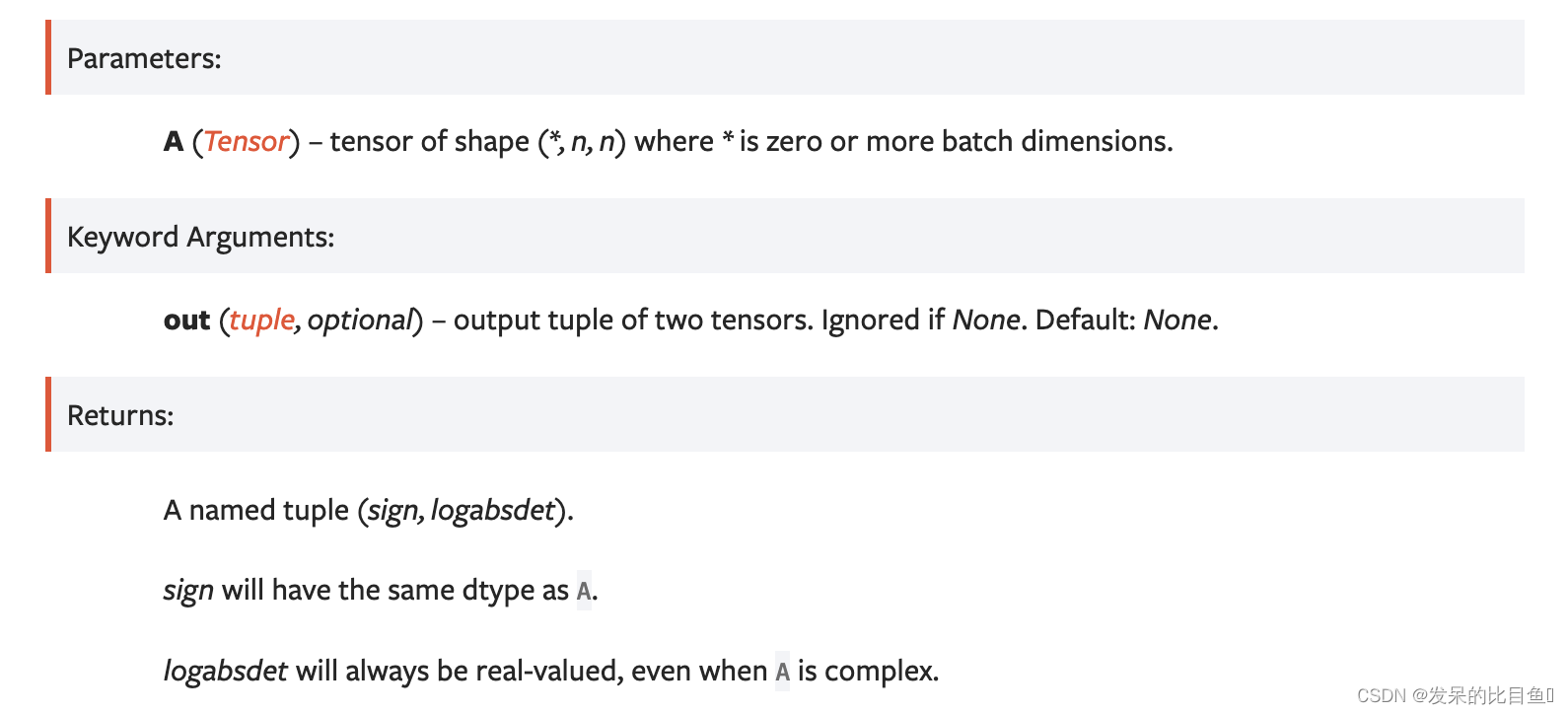
slogdet

torch.linalg.slogdet()的别名
计算一个平方矩阵的行列式的绝对值的符号和自然对数。
对于复数A，它返回行列式模的符号和自然对数，即行列式的对数极分解。
行列式可以恢复为符号*exp(logabsdet)。当矩阵的行列式为零时，它返回(0，-inf)。

>>> A = torch.randn(3, 3)
>>> A
tensor([[ 0.0032, -0.2239, -1.1219],
        [-0.6690,  0.1161,  0.4053],
        [-1.6218, -0.9273, -0.0082]])
>>> torch.linalg.det(A)
tensor(-0.7576)
>>> torch.logdet(A)
tensor(nan)
>>> torch.linalg.slogdet(A)
torch.return_types.linalg_slogdet(sign=tensor(-1.), logabsdet=tensor(-0.2776))

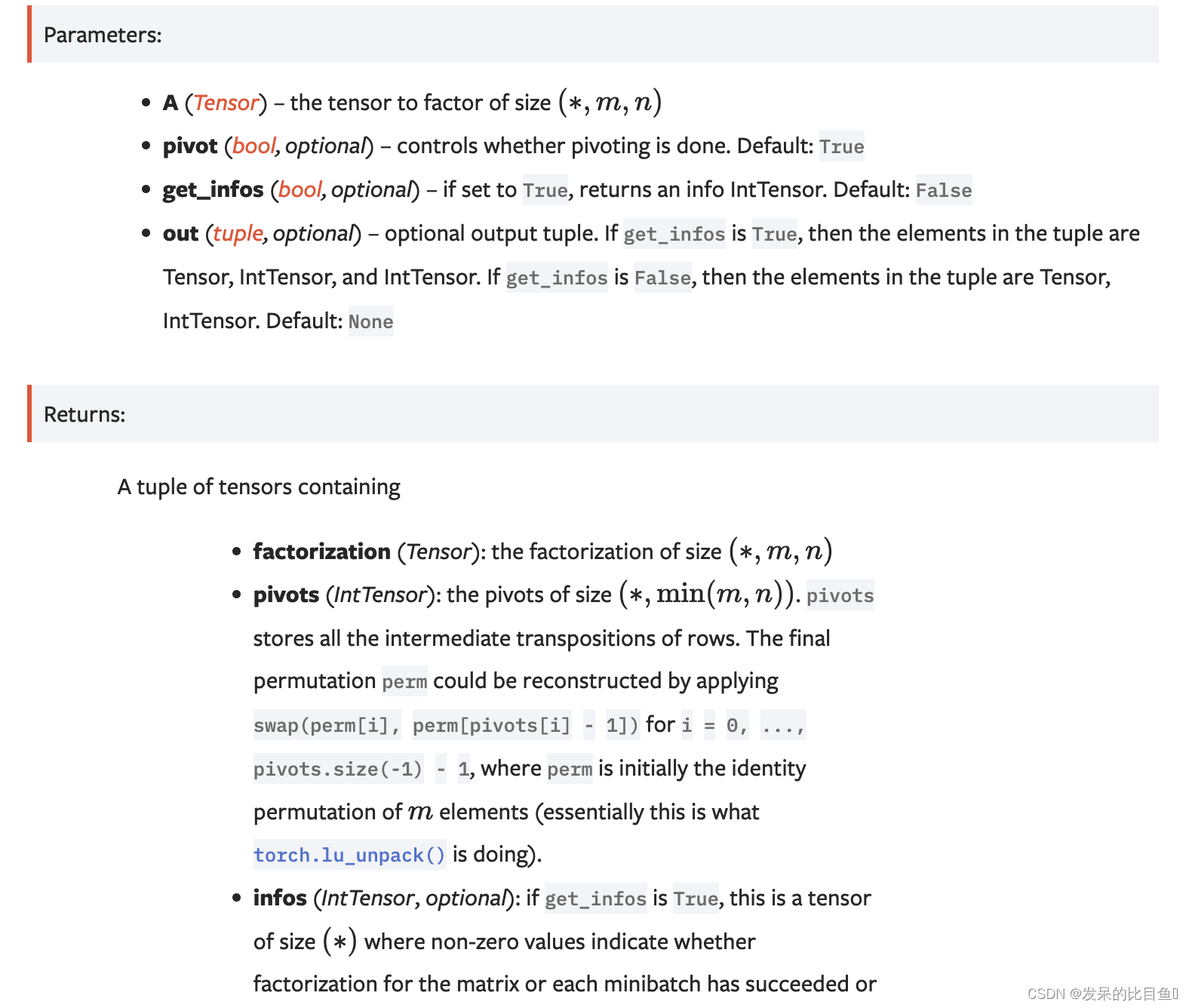
lu

计算一个矩阵或一批矩阵A的LU因子分解。返回一个包含LU因子分解和A的枢轴的元组。如果枢轴设置为True，则完成枢轴旋转。

>>> A = torch.randn(2, 3, 3)
>>> A_LU, pivots = torch.lu(A)
>>> A_LU
tensor([[[ 1.3506,  2.5558, -0.0816],
         [ 0.1684,  1.1551,  0.1940],
         [ 0.1193,  0.6189, -0.5497]],

        [[ 0.4526,  1.2526, -0.3285],
         [-0.7988,  0.7175, -0.9701],
         [ 0.2634, -0.9255, -0.3459]]])
>>> pivots
tensor([[ 3,  3,  3],
        [ 3,  3,  3]], dtype=torch.int32)
>>> A_LU, pivots, info = torch.lu(A, get_infos=True)
>>> if info.nonzero().size(0) == 0:
...     print('LU factorization succeeded for all samples!')
LU factorization succeeded for all samples!

lu_solve

使用LU_factor()中A的部分枢轴LU因子分解返回线性系统Ax=b的LU解。
此函数支持float、double、cfloat和cddouble数据类型的输入。

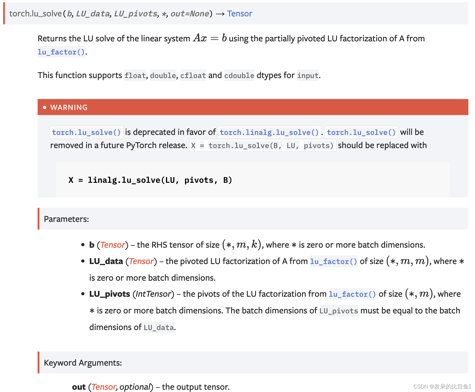
>>> A = torch.randn(2, 3, 3)
>>> b = torch.randn(2, 3, 1)
>>> LU, pivots = torch.linalg.lu_factor(A)
>>> x = torch.lu_solve(b, LU, pivots)
>>> torch.dist(A @ x, b)
tensor(1.00000e-07 *
       2.8312)

lu_unpack

将LU_factor()返回的LU分解解压为P、L、U矩阵。

>>> A = torch.randn(2, 3, 3)
>>> LU, pivots = torch.linalg.lu_factor(A)
>>> P, L, U = torch.lu_unpack(LU, pivots)
>>> # We can recover A from the factorization
>>> A_ = P @ L @ U
>>> torch.allclose(A, A_)
True

>>> # LU factorization of a rectangular matrix:
>>> A = torch.randn(2, 3, 2)
>>> LU, pivots = torch.linalg.lu_factor(A)
>>> P, L, U = torch.lu_unpack(LU, pivots)
>>> # P, L, U are the same as returned by linalg.lu
>>> P_, L_, U_ = torch.linalg.lu(A)
>>> torch.allclose(P, P_) and torch.allclose(L, L_) and torch.allclose(U, U_)
True

matmul

两个张量的矩阵乘积。

>>> # vector x vector
>>> tensor1 = torch.randn(3)
>>> tensor2 = torch.randn(3)
>>> torch.matmul(tensor1, tensor2).size()
torch.Size([])
>>> # matrix x vector
>>> tensor1 = torch.randn(3, 4)
>>> tensor2 = torch.randn(4)
>>> torch.matmul(tensor1, tensor2).size()
torch.Size([3])
>>> # batched matrix x broadcasted vector
>>> tensor1 = torch.randn(10, 3, 4)
>>> tensor2 = torch.randn(4)
>>> torch.matmul(tensor1, tensor2).size()
torch.Size([10, 3])
>>> # batched matrix x batched matrix
>>> tensor1 = torch.randn(10, 3, 4)
>>> tensor2 = torch.randn(10, 4, 5)
>>> torch.matmul(tensor1, tensor2).size()
torch.Size([10, 3, 5])
>>> # batched matrix x broadcasted matrix
>>> tensor1 = torch.randn(10, 3, 4)
>>> tensor2 = torch.randn(4, 5)
>>> torch.matmul(tensor1, tensor2).size()
torch.Size([10, 3, 5])

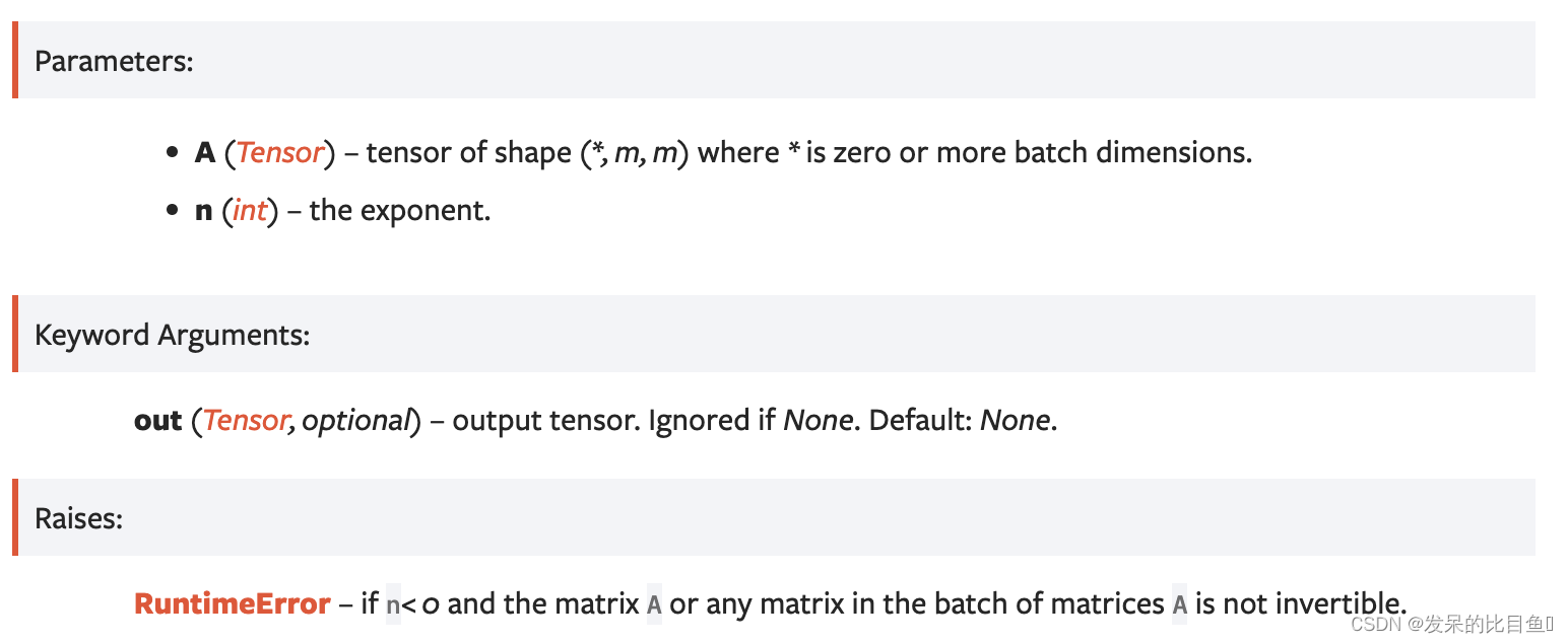
matrix_power

计算整数n的平方矩阵的n次方。

>>> A = torch.randn(3, 3)
>>> torch.linalg.matrix_power(A, 0)
tensor([[1., 0., 0.],
        [0., 1., 0.],
        [0., 0., 1.]])
>>> torch.linalg.matrix_power(A, 3)
tensor([[ 1.0756,  0.4980,  0.0100],
        [-1.6617,  1.4994, -1.9980],
        [-0.4509,  0.2731,  0.8001]])
>>> torch.linalg.matrix_power(A.expand(2, -1, -1), -2)
tensor([[[ 0.2640,  0.4571, -0.5511],
        [-1.0163,  0.3491, -1.5292],
        [-0.4899,  0.0822,  0.2773]],
        [[ 0.2640,  0.4571, -0.5511],
        [-1.0163,  0.3491, -1.5292],
        [-0.4899,  0.0822,  0.2773]]])

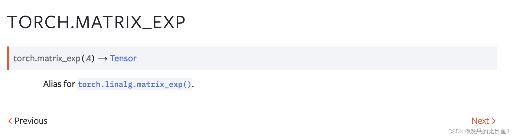
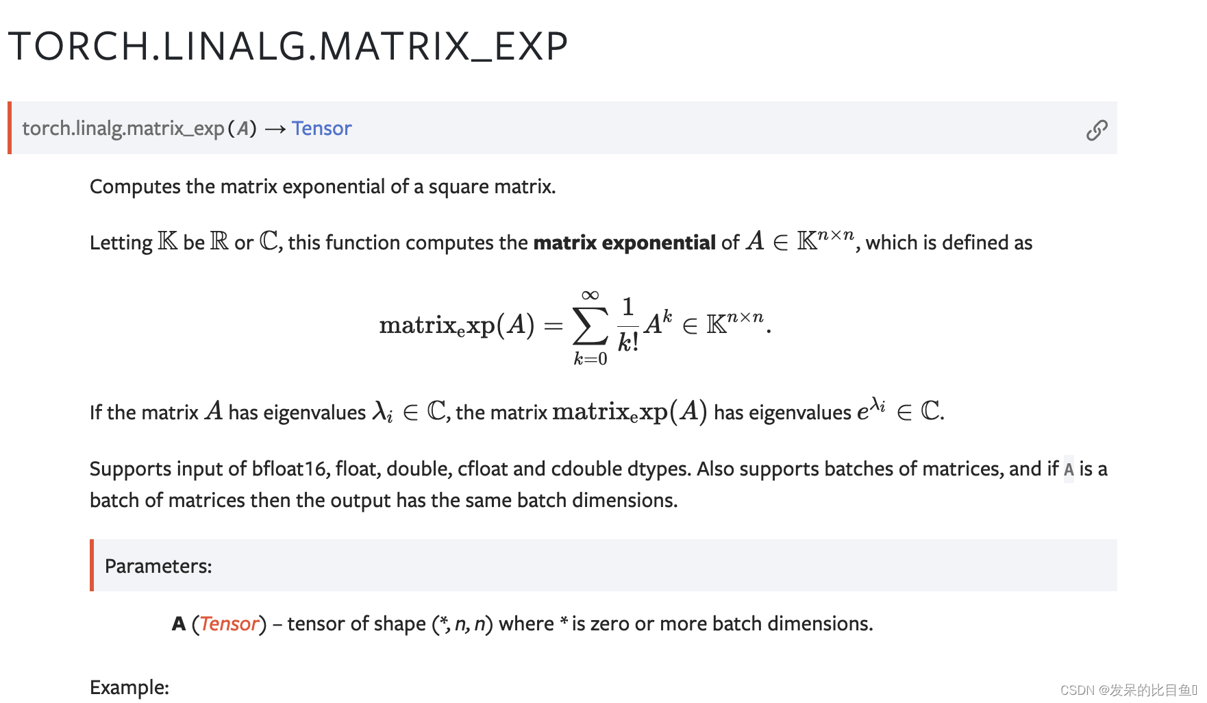
matrix_exp

计算平方矩阵的指数矩阵。

mm

对矩阵输入和mat2执行矩阵乘法运算。

>>> mat1 = torch.randn(2, 3)
>>> mat2 = torch.randn(3, 3)
>>> torch.mm(mat1, mat2)
tensor([[ 0.4851,  0.5037, -0.3633],
        [-0.0760, -3.6705,  2.4784]])

mv

执行矩阵输入和向量vec的矩阵向量乘积。

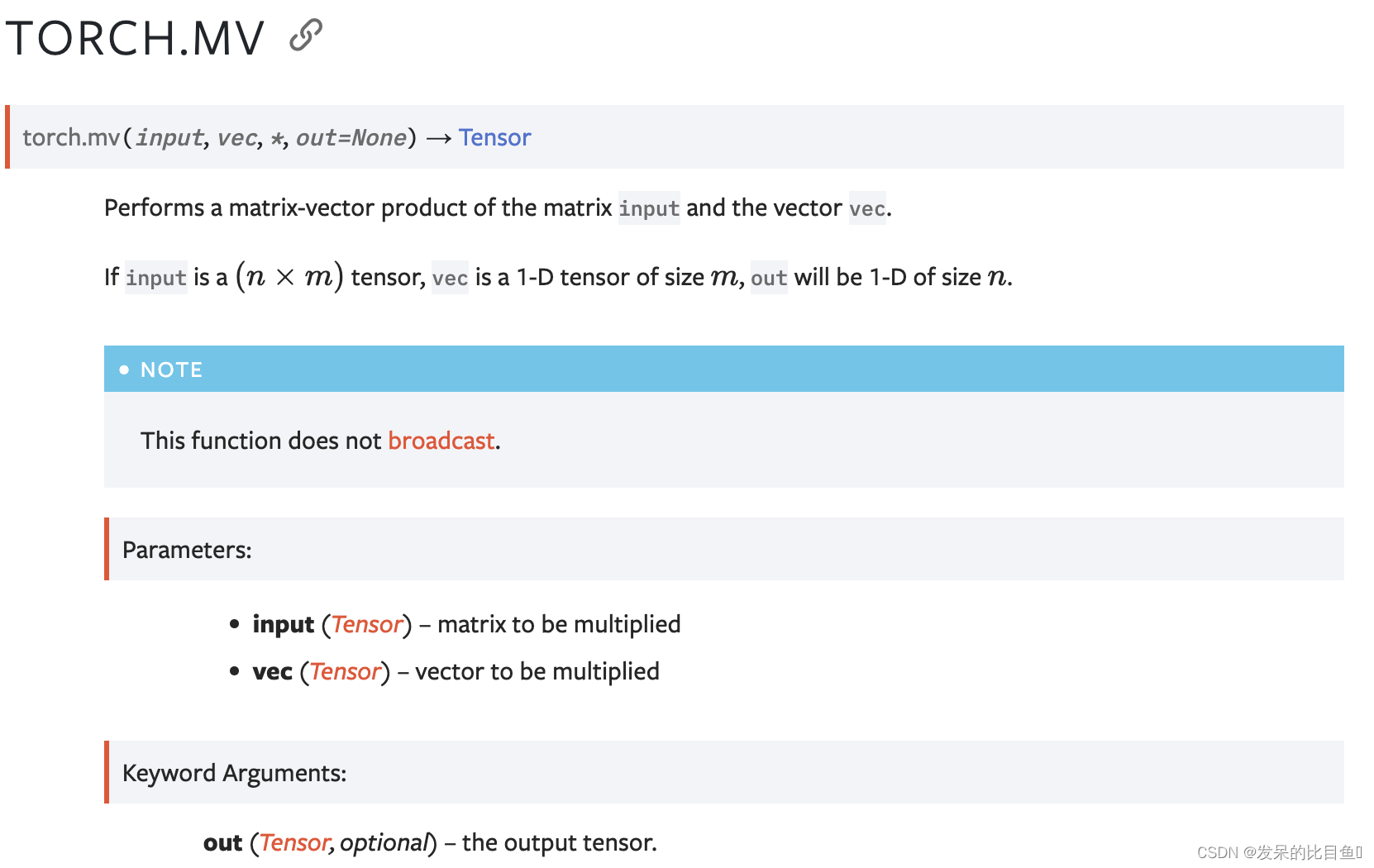
>>> mat = torch.randn(2, 3)
>>> vec = torch.randn(3)
>>> torch.mv(mat, vec)
tensor([ 1.0404, -0.6361])

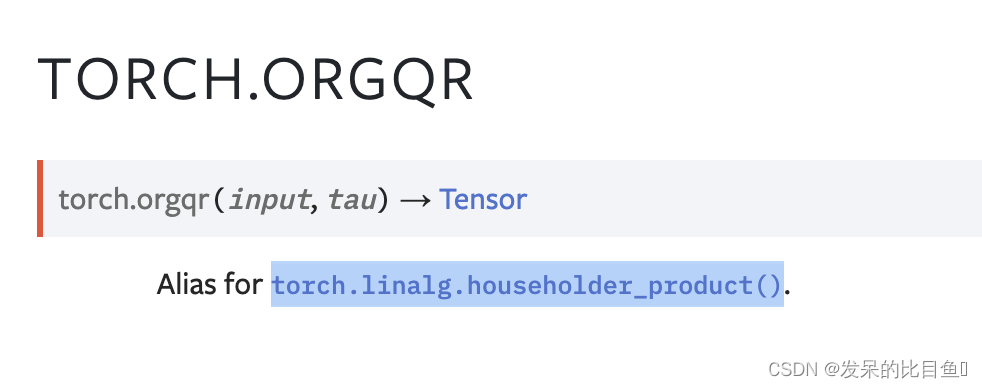
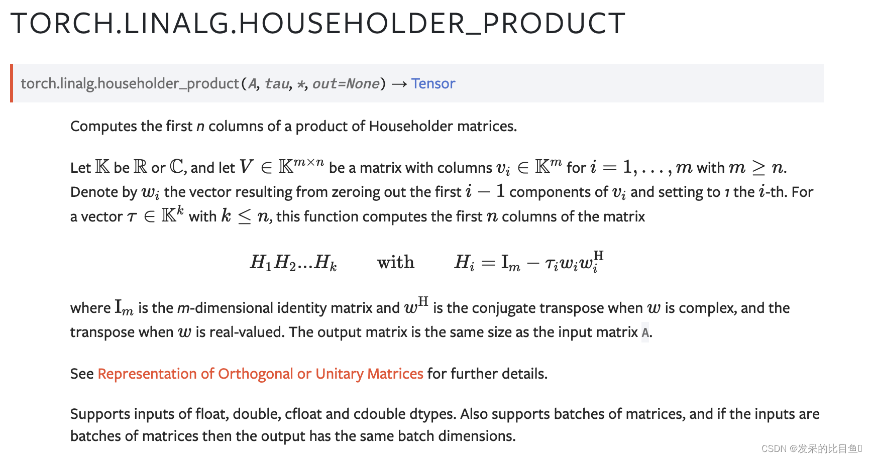
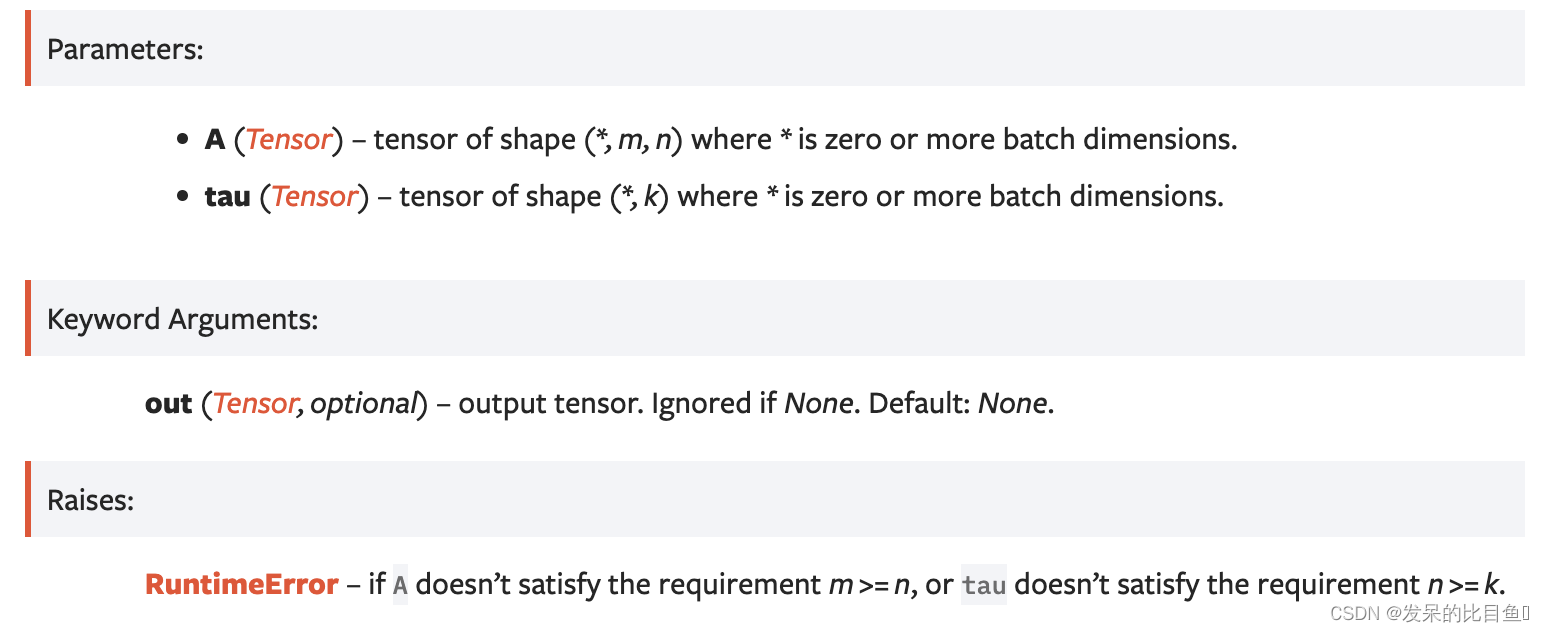
orgqr

torch.linear.householder_product()的别名。
计算Householder矩阵乘积的前n列。

>>> A = torch.randn(2, 2)
>>> h, tau = torch.geqrf(A)
>>> Q = torch.linalg.householder_product(h, tau)
>>> torch.dist(Q, torch.linalg.qr(A).Q)
tensor(0.)

>>> h = torch.randn(3, 2, 2, dtype=torch.complex128)
>>> tau = torch.randn(3, 1, dtype=torch.complex128)
>>> Q = torch.linalg.householder_product(h, tau)
>>> Q
tensor([[[ 1.8034+0.4184j,  0.2588-1.0174j],
        [-0.6853+0.7953j,  2.0790+0.5620j]],

        [[ 1.4581+1.6989j, -1.5360+0.1193j],
        [ 1.3877-0.6691j,  1.3512+1.3024j]],

        [[ 1.4766+0.5783j,  0.0361+0.6587j],
        [ 0.6396+0.1612j,  1.3693+0.4481j]]], dtype=torch.complex128)

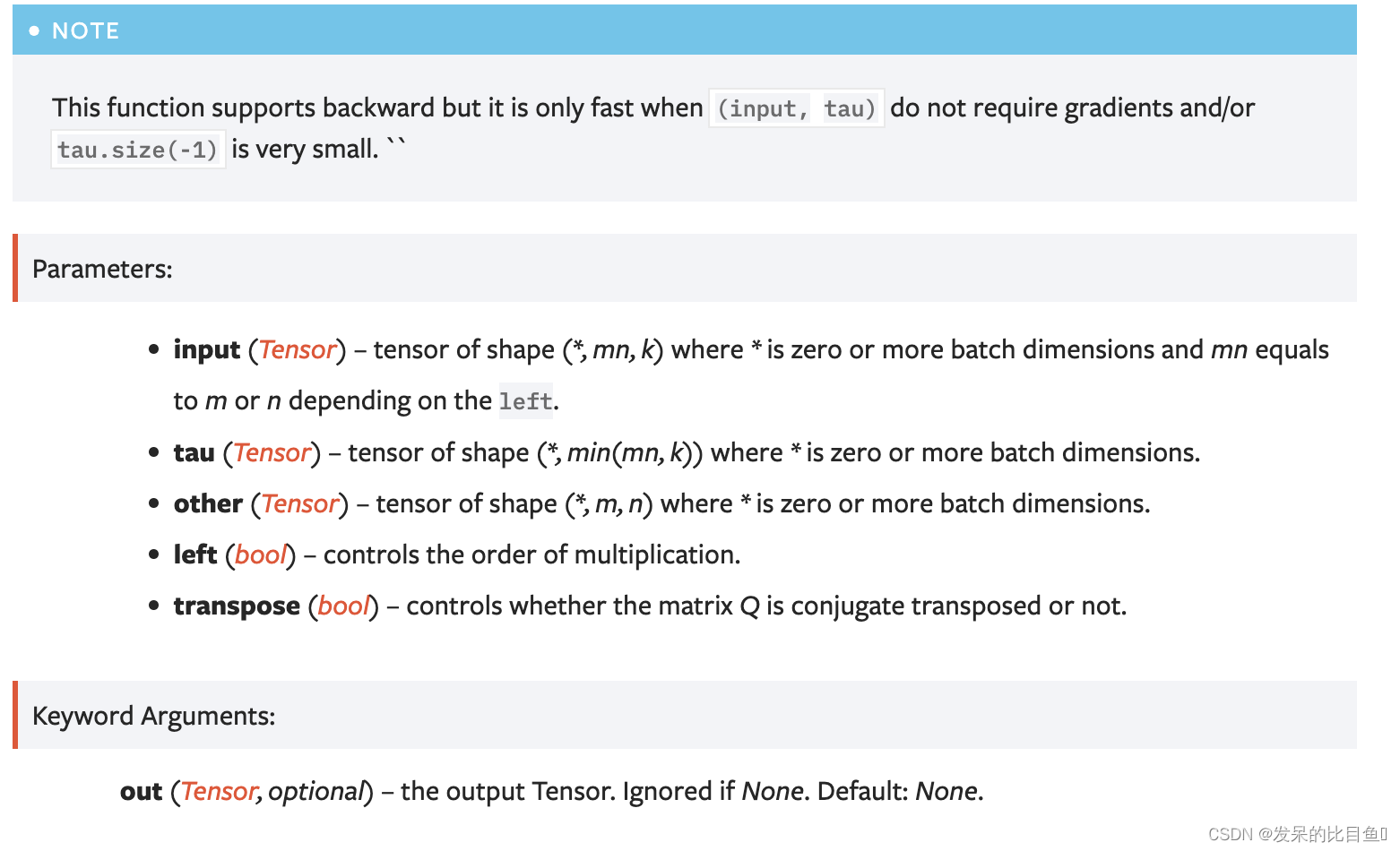
ormqr

计算Householder矩阵的乘积与一般矩阵的矩阵乘积。

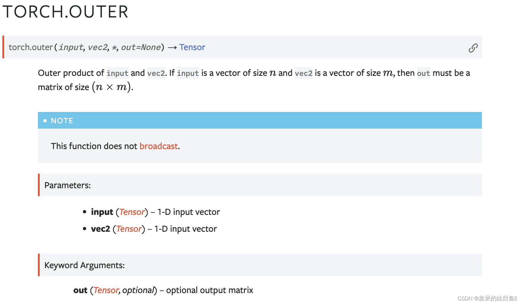
outer

输入和vec2的外积。如果input是大小为n的向量，vec2是大小为m的向量，那么out必须是大小为（n×m）的矩阵。

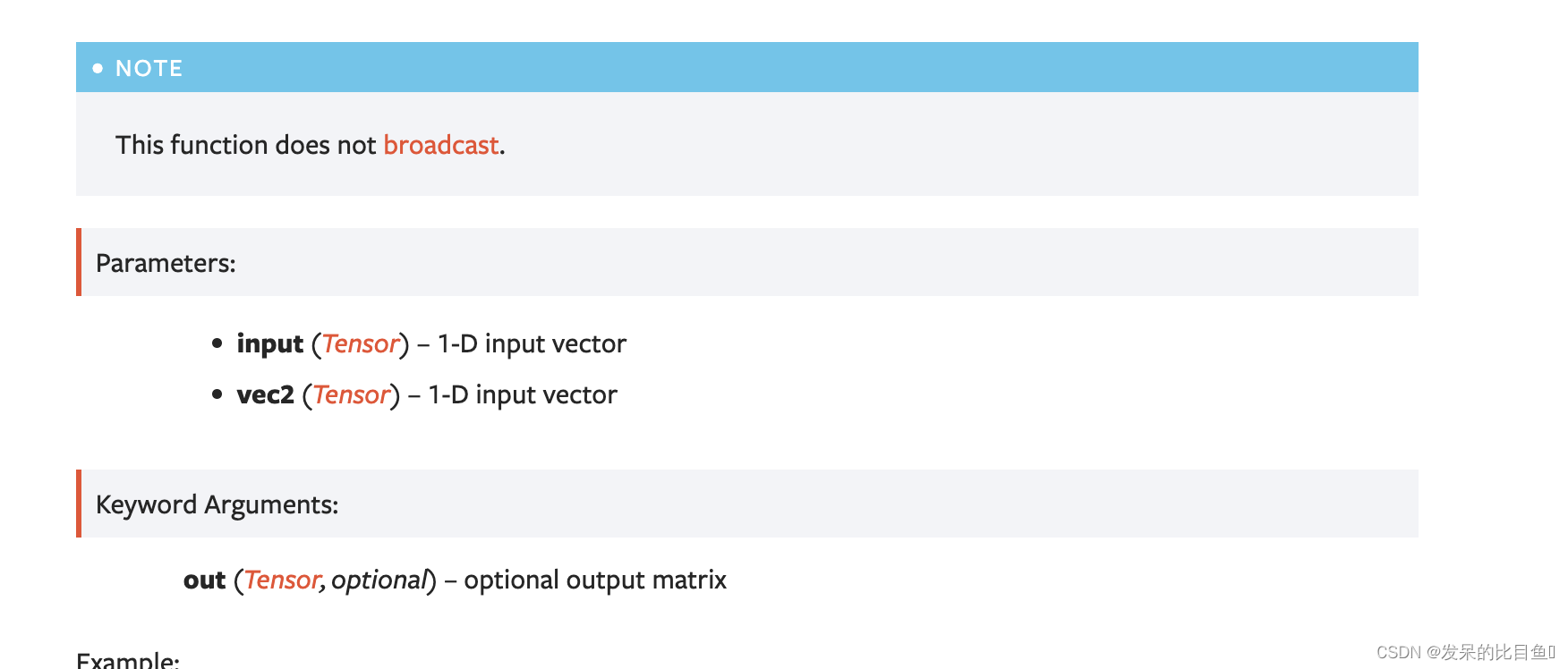
>>> v1 = torch.arange(1., 5.)
>>> v2 = torch.arange(1., 4.)
>>> torch.outer(v1, v2)
tensor([[  1.,   2.,   3.],
        [  2.,   4.,   6.],
        [  3.,   6.,   9.],
        [  4.,   8.,  12.]])

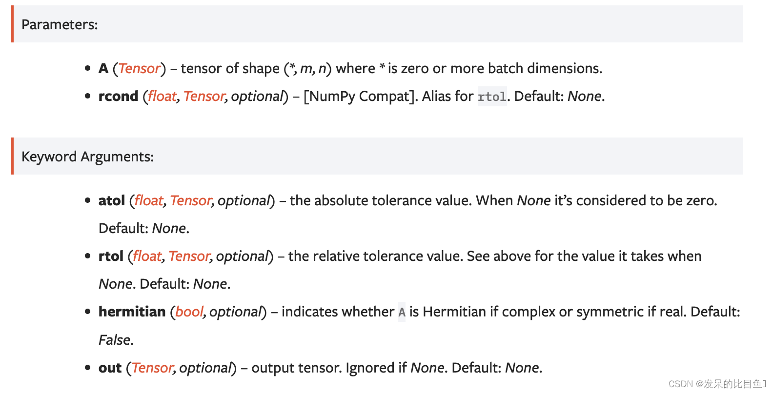
pinverse

torch.linalg.pinv()的别名
计算一个矩阵的伪逆(摩尔-彭罗斯逆)。

>>> A = torch.randn(3, 5)
>>> A
tensor([[ 0.5495,  0.0979, -1.4092, -0.1128,  0.4132],
        [-1.1143, -0.3662,  0.3042,  1.6374, -0.9294],
        [-0.3269, -0.5745, -0.0382, -0.5922, -0.6759]])
>>> torch.linalg.pinv(A)
tensor([[ 0.0600, -0.1933, -0.2090],
        [-0.0903, -0.0817, -0.4752],
        [-0.7124, -0.1631, -0.2272],
        [ 0.1356,  0.3933, -0.5023],
        [-0.0308, -0.1725, -0.5216]])

>>> A = torch.randn(2, 6, 3)
>>> Apinv = torch.linalg.pinv(A)
>>> torch.dist(Apinv @ A, torch.eye(3))
tensor(8.5633e-07)

>>> A = torch.randn(3, 3, dtype=torch.complex64)
>>> A = A + A.T.conj()  # creates a Hermitian matrix
>>> Apinv = torch.linalg.pinv(A, hermitian=True)
>>> torch.dist(Apinv @ A, torch.eye(3))
tensor(1.0830e-06)

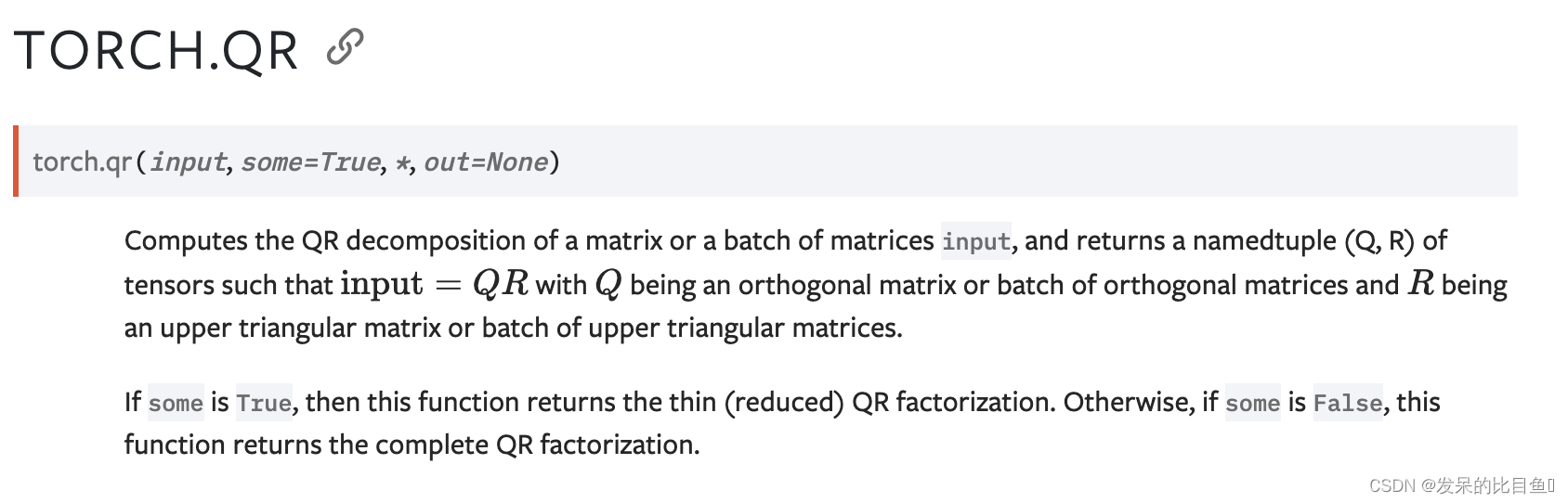
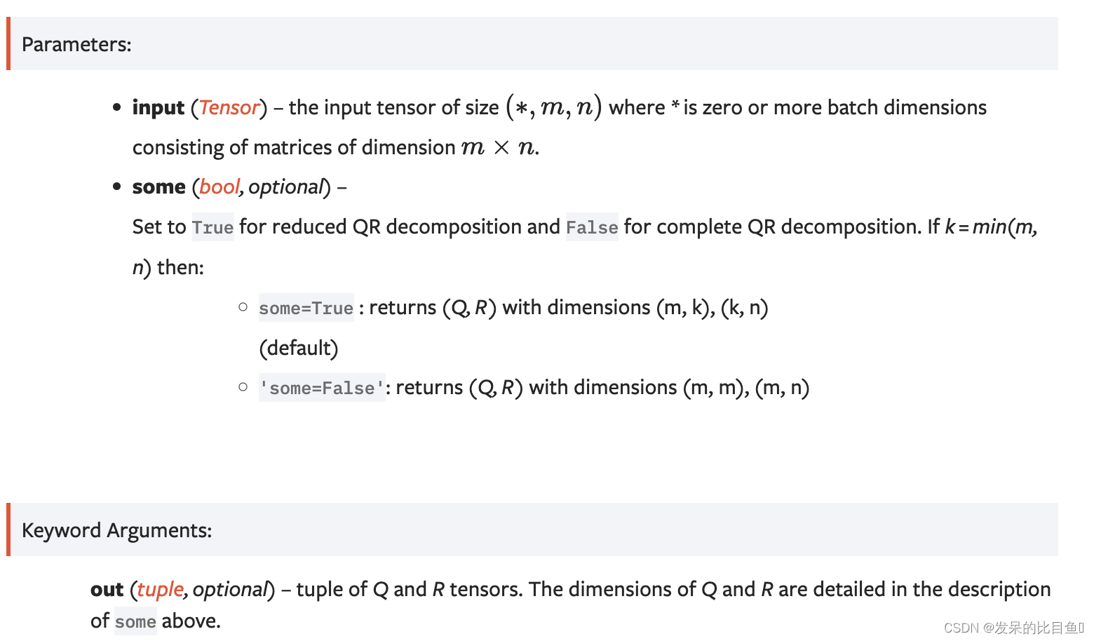
qr

计算输入的一个矩阵或一批矩阵的QR分解，并返回张量的命名元组（Q，R），使得input=QR，其中Q是正交矩阵或一组正交矩阵，R是上三角矩阵或上三角矩阵。

>>> a = torch.tensor([[12., -51, 4], [6, 167, -68], [-4, 24, -41]])
>>> q, r = torch.qr(a)
>>> q
tensor([[-0.8571,  0.3943,  0.3314],
        [-0.4286, -0.9029, -0.0343],
        [ 0.2857, -0.1714,  0.9429]])
>>> r
tensor([[ -14.0000,  -21.0000,   14.0000],
        [   0.0000, -175.0000,   70.0000],
        [   0.0000,    0.0000,  -35.0000]])
>>> torch.mm(q, r).round()
tensor([[  12.,  -51.,    4.],
        [   6.,  167.,  -68.],
        [  -4.,   24.,  -41.]])
>>> torch.mm(q.t(), q).round()
tensor([[ 1.,  0.,  0.],
        [ 0.,  1., -0.],
        [ 0., -0.,  1.]])
>>> a = torch.randn(3, 4, 5)
>>> q, r = torch.qr(a, some=False)
>>> torch.allclose(torch.matmul(q, r), a)
True
>>> torch.allclose(torch.matmul(q.mT, q), torch.eye(5))
True

svd

计算一个矩阵或一批矩阵输入的奇异值分解。奇异值分解表示为命名元组（U，S，V），使得输入=U diag（S）VH。其中VH是实数输入的V的转置，以及复数输入的V共轭转置。如果输入是一批矩阵，那么U、S和V也以与输入相同的批维度进行批处理。

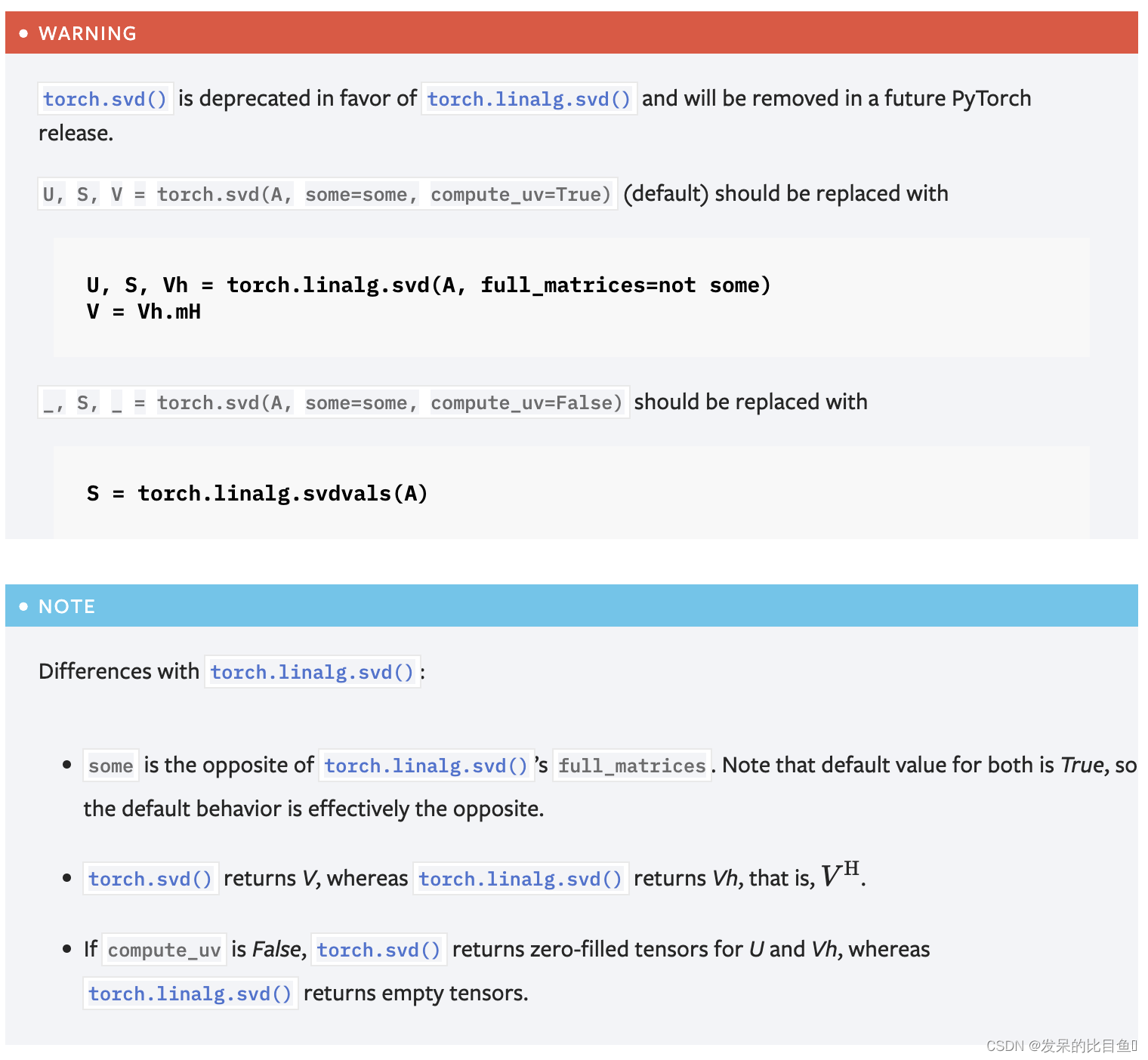
>>> a = torch.randn(5, 3)
>>> a
tensor([[ 0.2364, -0.7752,  0.6372],
        [ 1.7201,  0.7394, -0.0504],
        [-0.3371, -1.0584,  0.5296],
        [ 0.3550, -0.4022,  1.5569],
        [ 0.2445, -0.0158,  1.1414]])
>>> u, s, v = torch.svd(a)
>>> u
tensor([[ 0.4027,  0.0287,  0.5434],
        [-0.1946,  0.8833,  0.3679],
        [ 0.4296, -0.2890,  0.5261],
        [ 0.6604,  0.2717, -0.2618],
        [ 0.4234,  0.2481, -0.4733]])
>>> s
tensor([2.3289, 2.0315, 0.7806])
>>> v
tensor([[-0.0199,  0.8766,  0.4809],
        [-0.5080,  0.4054, -0.7600],
        [ 0.8611,  0.2594, -0.4373]])
>>> torch.dist(a, torch.mm(torch.mm(u, torch.diag(s)), v.t()))
tensor(8.6531e-07)
>>> a_big = torch.randn(7, 5, 3)
>>> u, s, v = torch.svd(a_big)
>>> torch.dist(a_big, torch.matmul(torch.matmul(u, torch.diag_embed(s)), v.mT))
tensor(2.6503e-06)

svd_lowrank

返回矩阵、矩阵批或稀疏矩阵A的奇异值分解(U, S, V)，使 $A≈Udiag(S)V^T$ 。在给定M的情况下，则计算矩阵A−M的SVD。

pca_lowrank

对低秩矩阵、此类矩阵的批或稀疏矩阵执行线性主成分分析（PCA）。

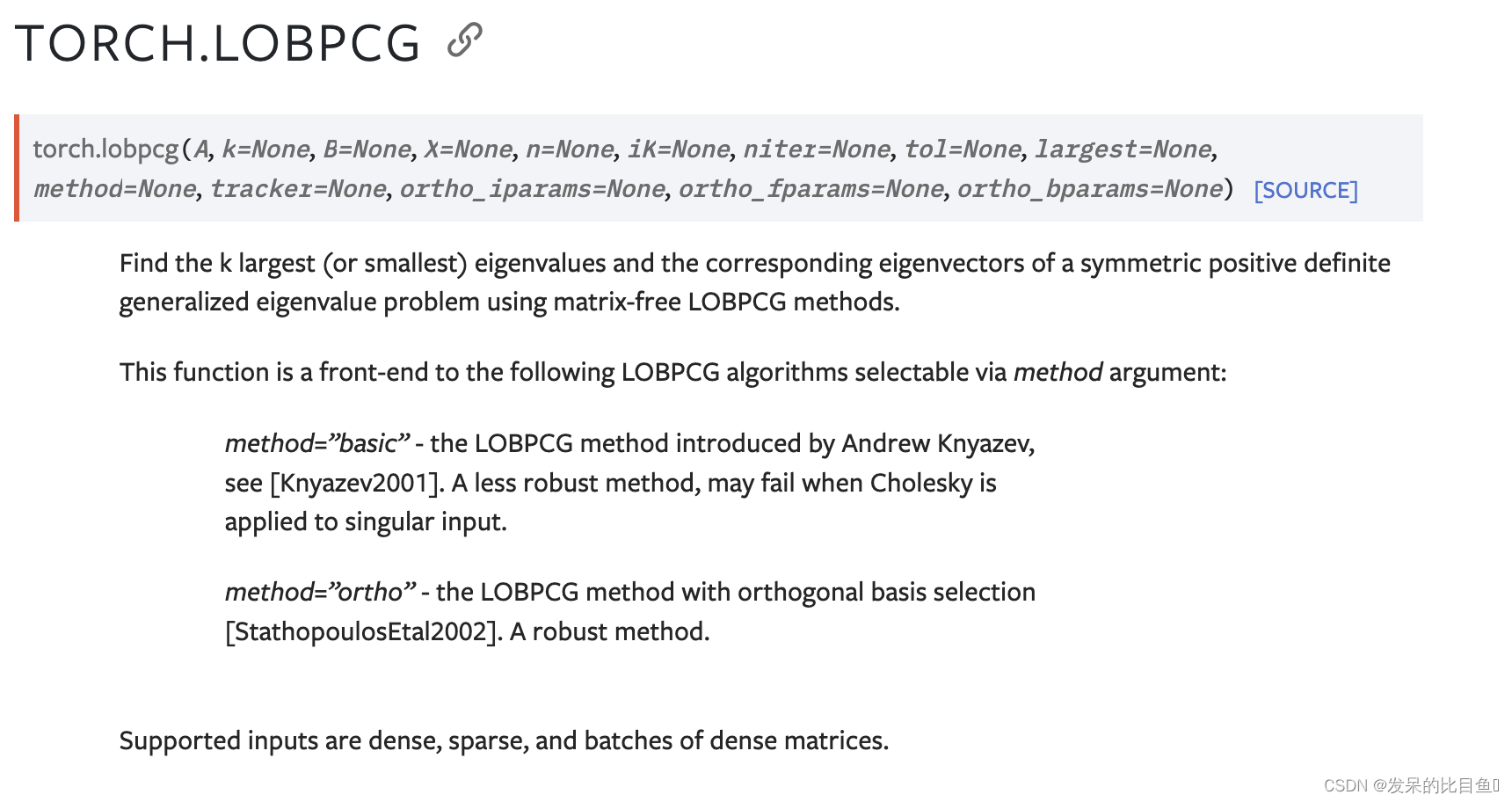
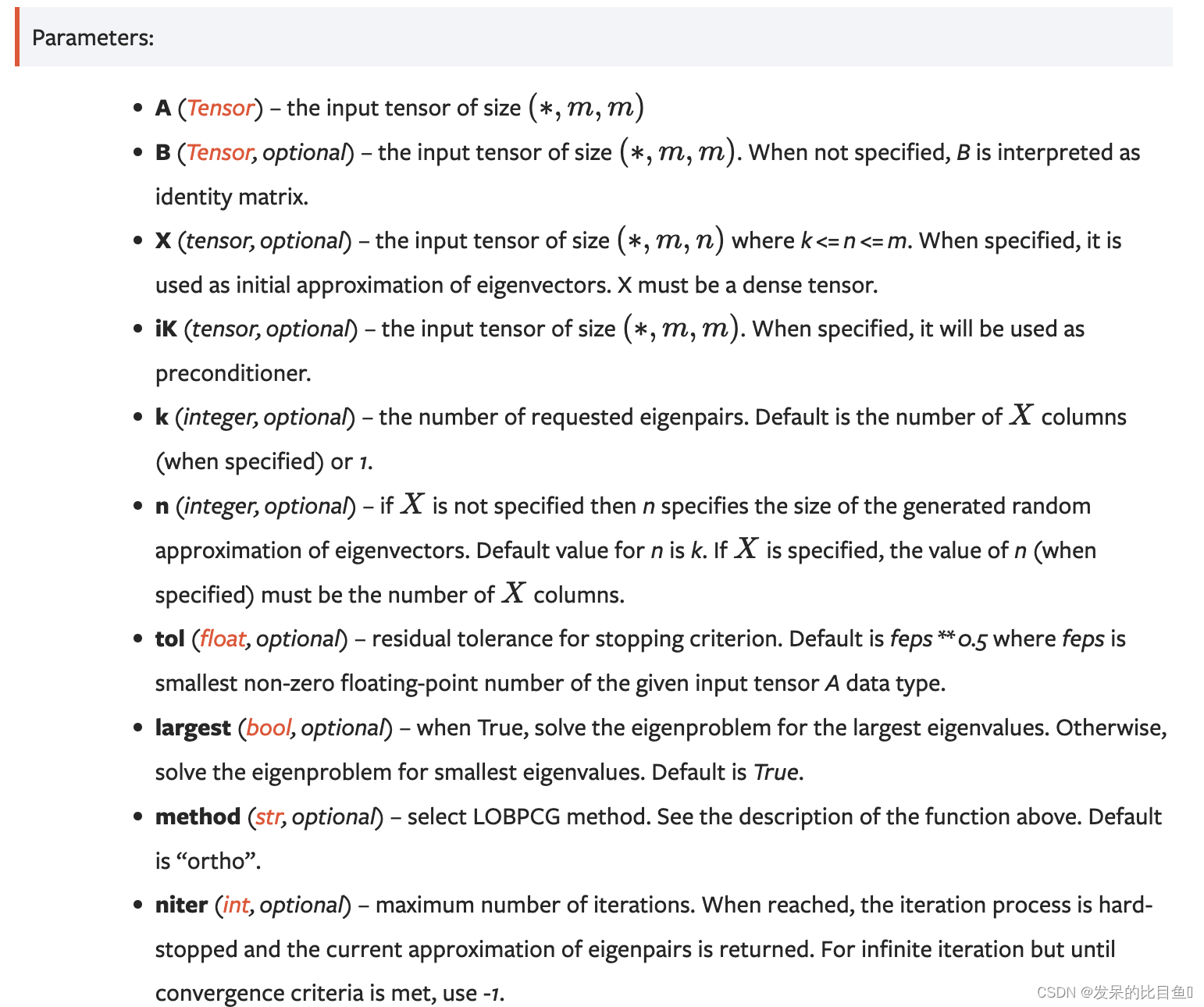
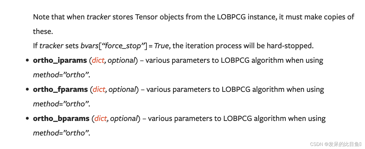
lobpcg

使用无矩阵LOBPCG方法找到对称正定广义特征值问题的k个最大（或最小）特征值和相应的特征向量。

trapz

torch.trapezoid().别名
沿dim计算梯形规则。默认情况下，假设元素之间的间距为1，但dx可用于指定不同的恒定间距，x可用于指定沿dim的任意间距。

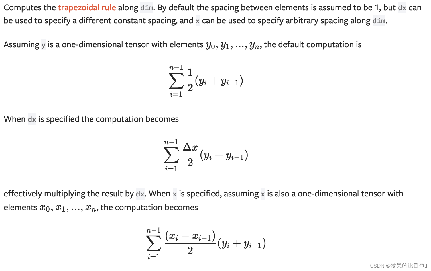
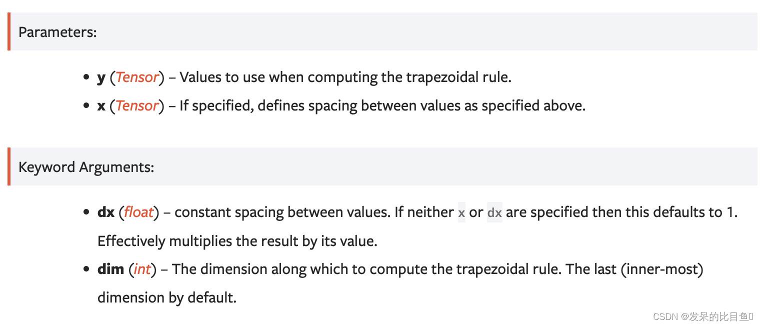
trapezoid

沿dim计算梯形规则。默认情况下，假设元素之间的间距为1，但dx可用于指定不同的恒定间距，x可用于指定沿dim的任意间距。

>>> # Computes the trapezoidal rule in 1D, spacing is implicitly 1
>>> y = torch.tensor([1, 5, 10])
>>> torch.trapezoid(y)
tensor(10.5)

>>> # Computes the same trapezoidal rule directly to verify
>>> (1 + 10 + 10) / 2
10.5

>>> # Computes the trapezoidal rule in 1D with constant spacing of 2
>>> # NOTE: the result is the same as before, but multiplied by 2
>>> torch.trapezoid(y, dx=2)
21.0

>>> # Computes the trapezoidal rule in 1D with arbitrary spacing
>>> x = torch.tensor([1, 3, 6])
>>> torch.trapezoid(y, x)
28.5

>>> # Computes the same trapezoidal rule directly to verify
>>> ((3 - 1) * (1 + 5) + (6 - 3) * (5 + 10)) / 2
28.5

>>> # Computes the trapezoidal rule for each row of a 3x3 matrix
>>> y = torch.arange(9).reshape(3, 3)
tensor([[0, 1, 2],
        [3, 4, 5],
        [6, 7, 8]])
>>> torch.trapezoid(y)
tensor([ 2., 8., 14.])

>>> # Computes the trapezoidal rule for each column of the matrix
>>> torch.trapezoid(y, dim=0)
tensor([ 6., 8., 10.])

>>> # Computes the trapezoidal rule for each row of a 3x3 ones matrix
>>> #   with the same arbitrary spacing
>>> y = torch.ones(3, 3)
>>> x = torch.tensor([1, 3, 6])
>>> torch.trapezoid(y, x)
array([5., 5., 5.])

>>> # Computes the trapezoidal rule for each row of a 3x3 ones matrix
>>> #   with different arbitrary spacing per row
>>> y = torch.ones(3, 3)
>>> x = torch.tensor([[1, 2, 3], [1, 3, 5], [1, 4, 7]])
>>> torch.trapezoid(y, x)
array([2., 4., 6.])

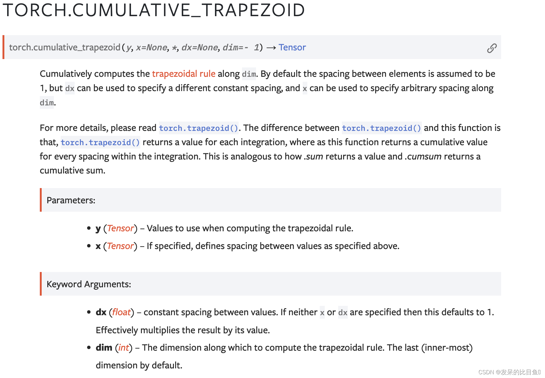
cumulative_trapezoid

沿着dim累积计算梯形规则。默认情况下，假设元素之间的间距为1，但dx可用于指定不同的恒定间距，x可用于指定沿dim的任意间距。

>>> # Cumulatively computes the trapezoidal rule in 1D, spacing is implicitly 1.
>>> y = torch.tensor([1, 5, 10])
>>> torch.cumulative_trapezoid(y)
tensor([3., 10.5])

>>> # Computes the same trapezoidal rule directly up to each element to verify
>>> (1 + 5) / 2
3.0
>>> (1 + 10 + 10) / 2
10.5

>>> # Cumulatively computes the trapezoidal rule in 1D with constant spacing of 2
>>> # NOTE: the result is the same as before, but multiplied by 2
>>> torch.cumulative_trapezoid(y, dx=2)
tensor([6., 21.])

>>> # Cumulatively computes the trapezoidal rule in 1D with arbitrary spacing
>>> x = torch.tensor([1, 3, 6])
>>> torch.cumulative_trapezoid(y, x)
tensor([6., 28.5])

>>> # Computes the same trapezoidal rule directly up to each element to verify
>>> ((3 - 1) * (1 + 5)) / 2
6.0
>>> ((3 - 1) * (1 + 5) + (6 - 3) * (5 + 10)) / 2
28.5

>>> # Cumulatively computes the trapezoidal rule for each row of a 3x3 matrix
>>> y = torch.arange(9).reshape(3, 3)
tensor([[0, 1, 2],
        [3, 4, 5],
        [6, 7, 8]])
>>> torch.cumulative_trapezoid(y)
tensor([[ 0.5,  2.],
        [ 3.5,  8.],
        [ 6.5, 14.]])

>>> # Cumulatively computes the trapezoidal rule for each column of the matrix
>>> torch.cumulative_trapezoid(y, dim=0)
tensor([[ 1.5,  2.5,  3.5],
        [ 6.0,  8.0, 10.0]])

>>> # Cumulatively computes the trapezoidal rule for each row of a 3x3 ones matrix
>>> #   with the same arbitrary spacing
>>> y = torch.ones(3, 3)
>>> x = torch.tensor([1, 3, 6])
>>> torch.cumulative_trapezoid(y, x)
tensor([[2., 5.],
        [2., 5.],
        [2., 5.]])

>>> # Cumulatively computes the trapezoidal rule for each row of a 3x3 ones matrix
>>> #   with different arbitrary spacing per row
>>> y = torch.ones(3, 3)
>>> x = torch.tensor([[1, 2, 3], [1, 3, 5], [1, 4, 7]])
>>> torch.cumulative_trapezoid(y, x)
tensor([[1., 2.],
        [2., 4.],
        [3., 6.]])

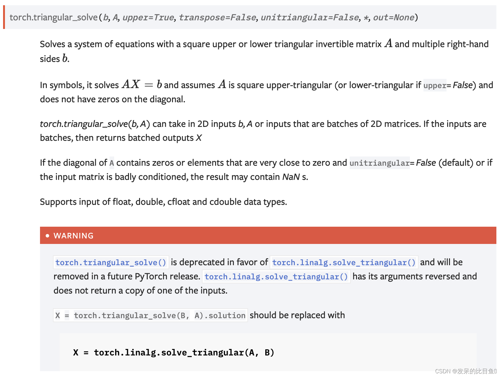
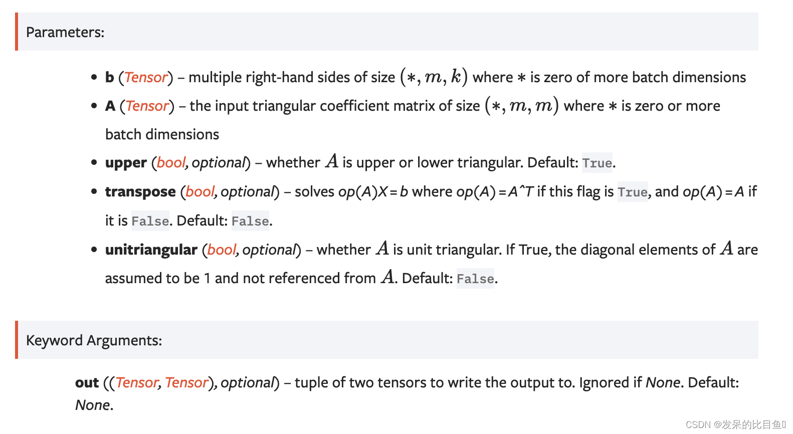
triangular_solve

求解具有正方形上或下三角形可逆矩阵A和多个右手边b的方程组。

>>> A = torch.randn(2, 2).triu()
>>> A
tensor([[ 1.1527, -1.0753],
        [ 0.0000,  0.7986]])
>>> b = torch.randn(2, 3)
>>> b
tensor([[-0.0210,  2.3513, -1.5492],
        [ 1.5429,  0.7403, -1.0243]])
>>> torch.triangular_solve(b, A)
torch.return_types.triangular_solve(
solution=tensor([[ 1.7841,  2.9046, -2.5405],
        [ 1.9320,  0.9270, -1.2826]]),
cloned_coefficient=tensor([[ 1.1527, -1.0753],
        [ 0.0000,  0.7986]]))

vdot

计算一个维度上两个1D向量的点积。

在符号中，此函数计算

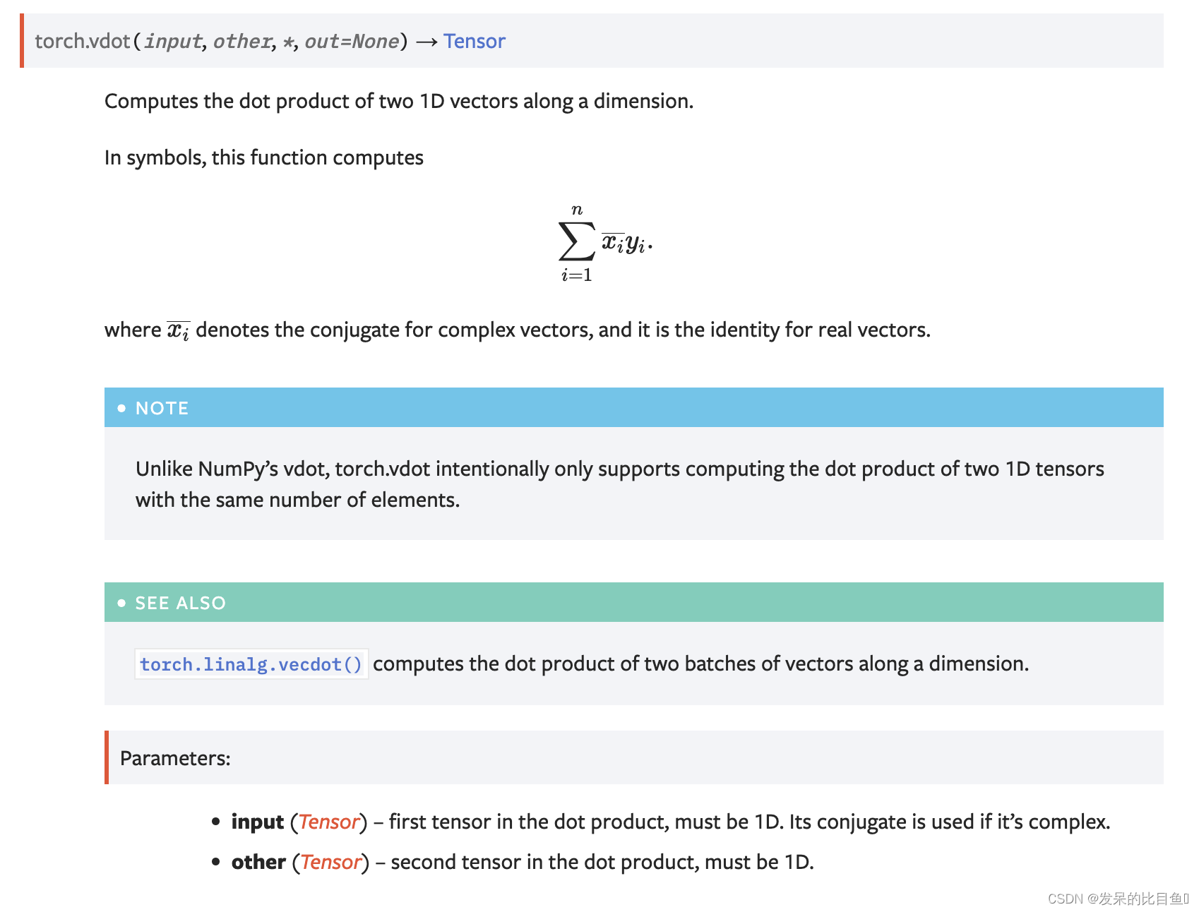
>>> torch.vdot(torch.tensor([2, 3]), torch.tensor([2, 1]))
tensor(7)
>>> a = torch.tensor((1 +2j, 3 - 1j))
>>> b = torch.tensor((2 +1j, 4 - 0j))
>>> torch.vdot(a, b)
tensor([16.+1.j])
>>> torch.vdot(b, a)
tensor([16.-1.j])

发呆的比目鱼

关注

0
点赞
踩
0

收藏

觉得还不错? 一键收藏
打赏
0
评论
小白学Pytorch系列--Torch API (10)

小白学Pytorch系列–Torch API (10)BLAS and LAPACK Operationsaddbmmaddmmaddmvaddrbaddbmmbmmchain_matmulcholeskycholesky_inversecholesky_solvedotgeqrfgerinnerinversedetlogdetslogdetlulu_solvelu_unpackmatmulmatmulmatrix_expmmmvorgqrormq
复制链接

扫一扫