经济增长模型

Douglas生产函数

用$Q(t),K(t),L(t)$分别表示某一地区或部门在时刻t的产值、资金和劳动
力，它们的关系可以一般地记作
$Q(t)=F(K(t),L(t))$
$z=Q/L,y=K/L$，z：产值，y：投资

$z=cg(y),g(y)=y^a,0<\alpha <1$
$Q=c{K}^{\alpha }{L}^{1-\alpha },0<\alpha <1$（Cobb-Douglas生产函数）

$\frac{\partial Q}{\partial K},\frac{\partial Q}{\partial L}>0,\frac{{\partial }^{2}Q}{\partial K^2},\frac{{\partial }^{2}Q}{\partial L^2}<0$
$\frac{K{Q}_K}{Q}=\alpha ,\frac{L{Q}_L}{Q}=1-\alpha ,K{Q}_K+L{Q}_L=Q$
$\alpha$是资金在产值中占有的份额，$1-\alpha$是劳动力在产值中占有的份额． 于是$\alpha$的大小直接反映了资金、劳动力二者对于创造产值的轻重
关系
$Q=c{K}^{\alpha }{L}^{\beta },0<\alpha ,\beta <1$

投资增长率与产值成正比，比例系数$\lambda$>0, 即用一定比例扩大再生产；
$\frac{\mathrm{d}K}{\mathrm{d}t}=\lambda Q,\lambda >0$
劳动力的相对增长率为常数$\mu$, ,$\mu$ 可以是负数，表示劳动力减少．
$\frac{\mathrm{d}L}{\mathrm{d}t}=\mu L$

$\frac{\mathrm{d}K}{\mathrm{d}t}=\lambda f_{0}L{y}^{\alpha }$
$\frac{\mathrm{d}K}{\mathrm{d}t}=L\frac{\mathrm{d}y}{\mathrm{d}t}+\mu Ly$
$\to \frac{\mathrm{d}y}{\mathrm{d}t}+\mu y=f_0\lambda y^{\alpha }$
$\to y(t)={\left(\frac{f_0\lambda }{\mu }+\left(y_0^{1-\alpha }-\frac{f_0\lambda }{\mu }\right){\mathrm{e}}^{-(1-\alpha )\mu t}\right)}^{1/1-\alpha }$
$y_0=K_0/L_0,Q_0=f_0{K}_0^{\alpha }{L}_0^{1-\alpha },{\dot{K}}_0=\lambda Q_0$
$$\to y(t)={\left\{\frac{f_0\lambda }{\mu }\left[1-\left(1-\mu \frac{K_0}{{\dot{K}}_0}\right)e^{-(1-\alpha )\mu t}\right]\right\}}^{\frac{1}{1-\alpha }}$$

$\frac{dy}{dt}+\mu y=c\lambda y^{\alpha }(0<\alpha <1)$
解析解：
$$y(t)={\left\{\frac{c\lambda }{\mu }\left[1-\left(1-\mu \frac{K_0}{{\dot{K}}_0}\right)e^{-(1-\alpha )\mu t}\right]\right\}}^{\frac{1}{1-\alpha }}$$

Bernoulli方程

$\frac{\mathrm{d}y}{\mathrm{d}x}+p(x)y=q(x)y^n$
两边除以$y^n$
$z=y^{1-n}$
$\frac{\mathrm{d}z}{\mathrm{d}x}+(1-n)p(x)z=(1-n)q(x)$

$\frac{\mathrm{d}y}{\mathrm{d}t}+\mu y=f_0\lambda y^{\alpha }$
$\to \frac{\mathrm{d}y}{\mathrm{d}t}\ast y^{-\alpha }+\mu y^{1-\alpha }=f_0\lambda$
$y^{1-\alpha }=z$
$\frac{dz}{dt}+\mu \ast z=f_0\lambda$

$Y(K,L)=K^{\alpha }\cdot L^{1-\alpha }$
$\frac{dY\left(K_0,L\right)}{dL}=(1-\alpha )\cdot K_0^{\alpha }\cdot L^{-\alpha }$

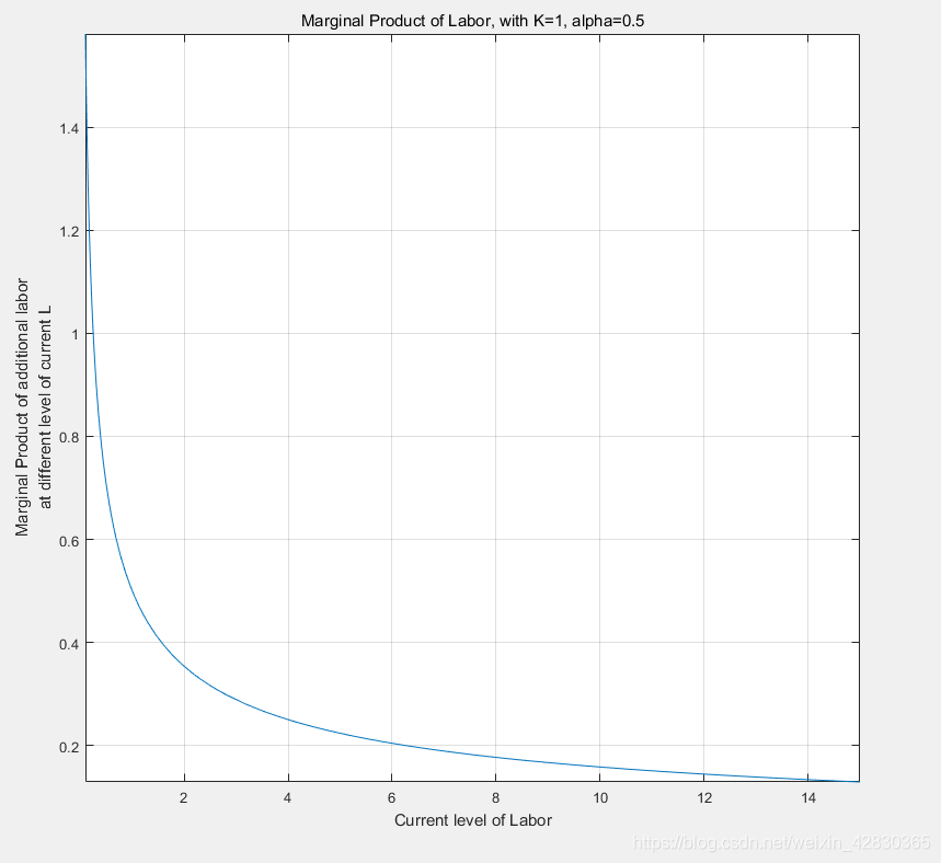
syms L K0 alpha
f(L, K0, alpha) = K0^(alpha)*L(1-alpha);
diff(f, L)

alpha = 0.5;
K0 = 1;
% Note that we have 1 symbolic variable now, the others are numbers
syms L
f(L) = K0^(alpha)*L(1-alpha);
f_diff_L = diff(f, L);
% Start figure
figure()
% fplot plots a function with one symbolic variable
fplot(f_diff_L, [0.1, 15])
title(‘Marginal Product of Labor, with K=1, alpha=0.5’)
ylabel({‘Marginal Product of additional labor’ ‘at different level of current L’})
xlabel(‘Current level of Labor’)
grid on

alpha = 0.5;
k0a = 1;
k0b = 2;
k0c = 3;
K0_vec = [k0a k0b k0c];
% Start figure
figure()
% Hold figure
hold on;
for K0 = K0_vec
% Note that we have 1 symbolic variable now, the others are numbers
syms L
f(L) = K0^(alpha)*L(1-alpha);
f_diff_L = diff(f, L);
% fplot plots a function with one symbolic variable
fplot(f_diff_L, [0.1, 15])
end
grid on
legend([‘k=’,num2str(k0a)],…
[‘k=’,num2str(k0b)],…
[‘k=’,num2str(k0c)]);
title(‘Marginal Product of Labor with different Capital Levels, alpha=0.5’)
ylabel({‘Marginal Product of additional labor’})
xlabel(‘Current level of Labor’)

% Define parameters and K0
alpha = 0.5;
beta = 0.5;
L0 = 1;
K = 1;
Y_at_L0 = (K^alpha)*(L0beta);
x_max = 5;
x_min = 0;
% a vector of h vectors
h_vec = [0.01, 1, 3];
% Loop over h, generate a plot for each rise over run as h changes
figure();
hold on;
% Legend
Legend_list = {};
% Plot as before the production function as a function of K
syms L
f(L) = (K^alpha)*(Lbeta);
fplot(f, [x_min, x_max], ‘LineWidth’, 2);
% Add to Legend List
legend_counter = 1;
Legend_list{1} = [‘Actual Line’];
% Plot the other lines
for h=h_vec
f_l0 = (K^alpha)*(L0beta);
f_l0_plus_h = (K^{alpha)*((L0+h)}beta);
2
% Current approximating line slope, based on formula above
cur_slope = (f_l0_plus_h - f_l0)/h;
% Current approximating line y-intercept, we require line to cross (K0, Y_at_K0), and know slope already
cur_y_intercept = Y_at_L0 - cur_slopeL0;
% Plot each of the approximating Slopes
syms L
f(L) = cur_y_intercept + cur_slopeL;
fplot(f, [x_min, x_max], ‘–’);
plot([h+L0, h+L0], ylim, ‘-k’);
% Legend
legend_counter = 1 + legend_counter;
Legend_list{legend_counter} = [‘h=’ num2str(h) ‘, slope=’ num2str(cur_slope)];
end
grid on;
ylabel(‘Cobb-Douglas Output’);
xlabel(‘Labor’);
title({‘Tangent line as h gets smaller’…
,[‘Output with Increasing Labor, fixed Capital=’ num2str(K)]})
legend(Legend_list,‘Location’, ‘NW’,‘Orientation’ ,‘Vertical’ );

% a bigger evenly spaced vector of h
h_grid_count = 100;
h = linspace(0, 15, h_grid_count);
% output at f_x0_plus_h
x0_plus_h = L0+h;
f_x0 = (K^alpha)*(L0.beta);
f_x0_plus_h = (K^{alpha)*((x0_plus_h).}beta);
% average output per additional worker
f_prime_x0 = (f_x0_plus_h - f_x0)./h;
3
% Store Results in a Table
T = table(h’, x0_plus_h’, f_x0_plus_h’, f_prime_x0’);
T.Properties.VariableNames = {‘h’, ‘x0_plus_h’, ‘f_x0_plus_h’, ‘f_prime_x0’};
% Graph
close all;
figure();
plot(h, f_prime_x0);
grid on;
ylabel(‘Average output increase per unit of labor increase’)
xlabel(‘h=increases in labor from L=2 (K=1 fixed)’)
title(‘Derivative Approximation as h gets small, CD Production’)

$\frac{\mathrm{d}y}{\mathrm{d}t}+\mu y=f_0\lambda y^{\alpha }$
$\to \frac{\mathrm{d}y}{\mathrm{d}t}\ast y^{-\alpha }+\mu y^{1-\alpha }=f_0\lambda$
$y^{1-\alpha }=z$
$\frac{dz}{dt}+\mu \ast z=f_0\lambda$

$\alpha =0.5,K_0=1,L_0=1,\lambda =1,\mu =1,f_0=1$
$\frac{dL}{dt}=L$
$\frac{dz}{dt}+z=1,z_0=1$

tspan = [0 100];
y0 = 1;
[t,y] = ode45(@(t,y) 1-y, tspan, y0);
plot(t,y,’-o’)

tspan = [0 100];
y0 = 1;
[t,y] = ode45(@(t,y) 1+y, tspan, y0);
plot(t,y,’-o’)

$\alpha =0.5,K_0=1,L_0=1,\lambda =1,\mu =-1,f_0=1$
$\frac{dL}{dt}=L$
$\frac{dz}{dt}-z=1,z_0=1$

tspan = [0 10];

t	z
0.0001	0.0004
0.0001	0.0005
0.0001	0.0006
0.0002	0.0008
0.0002	0.0011
0.0002	0.0014
0.0002	0.0018
0.0003	0.0024
0.0003	0.0030
0.0003	0.0039
0.0003	0.0051
0.0004	0.0066
0.0004	0.0085
0.0004	0.0109
0.0004	0.0140
0.0005	0.0180
0.0005	0.0232
0.0005	0.0298
0.0005	0.0382
0.0006	0.0491
0.0006	0.0631
0.0006	0.0811
0.0006	0.1041
0.0007	0.1337
0.0007	0.1717
0.0007	0.2205
0.0007	0.2832
0.0008	0.3636
0.0008	0.4670
0.0008	0.5996
0.0008	0.7699
0.0009	0.9887
0.0009	1.2697
0.0009	1.6302
0.0009	2.0931
0.0010	2.6877
0.0010	3.0412
0.0010	3.4412
0.0010	3.8938
0.0010	4.4059