[Modern Robotics] 4 -机器人正向运动

正向运动

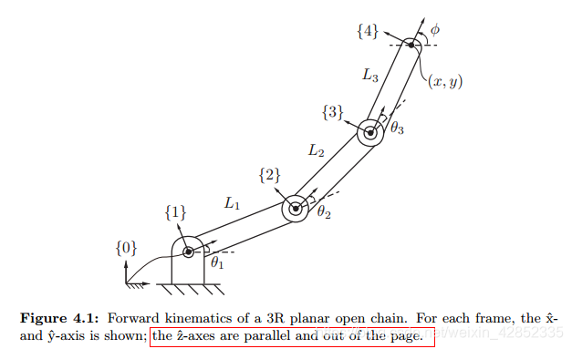
正向运动是指根据给定的关节转角 $\theta$ 来计算末端执行器的位置与方向。图4.1展示了一个3R平面开链式机械臂的正向运动问题。连杆的长度分别为 $L_1,L_2,L_3$。选取 { 0 } \{0\} {0}为固定坐标系，原点与基关节重合，并且假设坐标系 { 4 } \{4\} {4}固连于第三个连杆的顶部。则末端执行器的位置和方向可以计算如下：

$$\begin{array}{rl}x& =L_{1}cos{\theta }_1+L_{2}cos({\theta }_1+{\theta }_2)+L_{3}cos({\theta }_1+{\theta }_2+{\theta }_3)\\ y& =L_{1}sin{\theta }_1+L_{2}sin({\theta }_1+{\theta }_2)+L_{3}sin({\theta }_1+{\theta }_2+{\theta }_3)\\ \varphi & ={\theta }_1+{\theta }_2+{\theta }_3\end{array}$$
一种更系统的方法是在每个连杆上都固连一个坐标系，如图4.1的 { 1 } \{1\} {1}， { 2 } \{2\} {2}， { 3 } \{3\} {3}。这样，正向运动可以写成四个齐次变换矩阵的乘积：
$$T_{04}=T_{01}{T}_{12}{T}_{23}{T}_{34}\text{\hspace{1em}(4.4)}$$
其中，
$$\begin{array}{rl}{T}_{01}& =\left[\begin{array}{cccc}cos{\theta }_1& -sin{\theta }_1& 0& 0\\ sin{\theta }_1& cos{\theta }_1& 0& 0\\ 0& 0& 1& 0\\ 0& 0& 0& 1\end{array}\right],T_{12}=\left[\begin{array}{cccc}cos{\theta }_2& -sin{\theta }_2& 0& L_1\\ sin{\theta }_2& cos{\theta }_2& 0& 0\\ 0& 0& 1& 0\\ 0& 0& 0& 1\end{array}\right],\\ T_{23}& =\left[\begin{array}{cccc}cos{\theta }_3& -sin{\theta }_3& 0& L_2\\ sin{\theta }_3& cos{\theta }_3& 0& 0\\ 0& 0& 1& 0\\ 0& 0& 0& 1\end{array}\right],T_{34}=\left[\begin{array}{cccc}1& 0& 0& L_3\\ 0& 1& 0& 0\\ 0& 0& 1& 0\\ 0& 0& 0& 1\end{array}\right].\end{array}\text{\hspace{1em}(4.5)}$$
注意到，$T_{34}$ 是常量，并且 $T_{i-1,i}$ 只依赖于关节转角 ${\theta }_i$。

另一种方法，我们把所有关节转角为0时的末端执行器的位置和方向定义为 $M$ 矩阵，则有：
$$M=\left[\begin{array}{cccc}1& 0& 0& L_1+L_2+L_3\\ 0& 1& 0& 0\\ 0& 0& 1& 0\\ 0& 0& 0& 1\end{array}\right],\text{\hspace{1em}(4.6)}$$
现在我们把每个旋转轴关节当作为一个零螺距的旋量轴。假设 ${\theta }_1$ 与 ${\theta }_2$ 均为0，那么绕关节 3 旋转的旋量轴在 { 0 } \{0\} {0}坐标系的表示为：
$${\mathcal{S}}_3=\left[\begin{array}{c}{w}_3\\ v_3\end{array}\right]=\left[\begin{array}{c}0\\ 0\\ 1\\ 0\\ -(L_1+L_2)\\ 0\end{array}\right]$$
其中，$v_3=-w_3\times q_3$，$q_3$ 是在坐标系 { 0 } \{0\} {0}下的关节3旋转轴上的任一点，比如 $q_3=(L_1+L_2,0,0)$。
旋量轴 ${\mathcal{S}}_3$ 可以用 $se(3)$下的矩阵形式表示为：
$$[{\mathcal{S}}_3]=\left[\begin{array}{cc}[w]& v\\ 0& 0\end{array}\right]=\left[\begin{array}{cccc}0& -1& 0& 0\\ 1& 0& 0& -(L_1+L_2)\\ 0& 0& 0& 0\\ 0& 0& 0& 0\end{array}\right].$$
对于任意的 ${\theta }_3$，旋量运动的矩阵指数表示可以写成：
$$T_{04}=e^{[{\mathcal{S}}_3]{\theta }_3}M(for{\theta }_1={\theta }_2=0)\text{\hspace{1em}(4.7)}$$
现在让 ${\theta }_1=0$ ，任意固定的 ${\theta }_3$，绕着关节2的旋转可以看作这样的旋量运动：
$$T_{04}=e^{[{\mathcal{S}}_2]{\theta }_2}{e}^{[{\mathcal{S}}_3]{\theta }_3}M(for{\theta }_1=0)\text{\hspace{1em}(4.8)}$$
其中，$[{\mathcal{S}}_3],M$ 在前面已经定义，
$$[{\mathcal{S}}_2]=\left[\begin{array}{cccc}0& -1& 0& 0\\ 1& 0& 0& -L_1\\ 0& 0& 0& 0\\ 0& 0& 0& 0\end{array}\right].\text{\hspace{1em}(4.9)}$$
最终，让${\theta }_2$，${\theta }_3$ 保持固定，绕关节1的旋转可以认为是整个刚体连杆体的旋量运动。有：
$$T_{04}=e^{[{\mathcal{S}}_1]{\theta }_1}{e}^{[{\mathcal{S}}_2]{\theta }_2}{e}^{[{\mathcal{S}}_3]{\theta }_3}M\text{\hspace{1em}(4.10)}$$
其中：
$$[{\mathcal{S}}_1]=\left[\begin{array}{cccc}0& -1& 0& 0\\ 1& 0& 0& 0\\ 0& 0& 0& 0\\ 0& 0& 0& 0\end{array}\right].\text{\hspace{1em}(4.11)}$$
注意到，这里仅定义了 { 0 } \{0\} {0}坐标系与 $M$。这种方法叫做product of exponentials(PoE)区别于DH参数法。详情需了解DH参数法。

指数公式的乘积

使用 $PoE$ 公式，只需要指定一个固定坐标系 { s } \{s\} {s}（比如固结于机器人的固定基座），与各关节均在零位时的末端执行器的坐标系 { b } \{b\} {b}，用 $M$ 来表示。

第一个公式：在固定坐标系下的旋量轴

$PoE$ 公式的关键概念是把每个关节当做在所有连杆上的旋量运动。如图4.2所示的通用开式链，由 $n$ 个自由度为1的关节链接而成。固定坐标系选取如图。$M\in SE(3)$ 来表示零位状态下末端坐标系相对于固定坐标系的位置与方向。

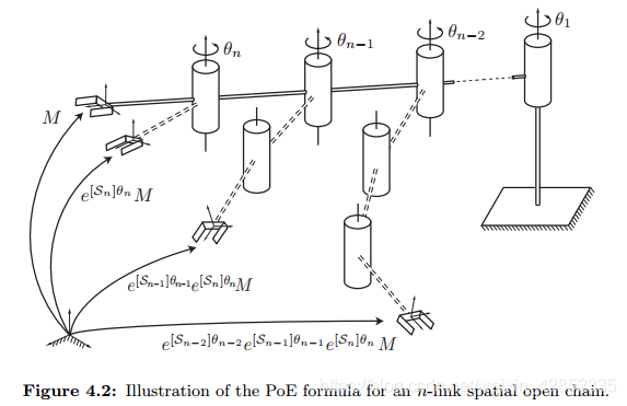
现在假设关节 $n$ 转动了 ${\theta }_n$ 角度，则末端的 $M$ 经历了一个如下形式的移动：
$$T=e^{[{\mathcal{S}}_n]{\theta }_n}M\text{\hspace{1em}(4.12)}$$
其中，$T\in SE(3)$，是末端执行器新的方位，${\mathcal{S}}_n=(w_n,v_n)$ 是固定坐标系下关节 $n$ 的旋量轴。
假设关节 $n-1$ 也变化，那就相当于在连杆 $n-1$ 上施加一个旋量运动，如下：
$$T=e^{[{\mathcal{S}}_{n-1}]{\theta }_{n-1}}{e}^{[{\mathcal{S}}_n]{\theta }_n}M\text{\hspace{1em}(4.13)}$$
继续这样的过程，可以得到：
$$T=e^{[{\mathcal{S}}_1]{\theta }_1}\cdots e^{[{\mathcal{S}}_{n-1}]{\theta }_{n-1}}{e}^{[{\mathcal{S}}_n]{\theta }_n}M\text{\hspace{1em}(4.14)}$$
上式即描述了一个 $n$ 自由度的开式链的指数公式乘积。注意前提是旋量轴在表达在固定坐标系的。

应用公式需要的量总结如下：

1. 机器人在零位时的末端执行器的方位 $M\in SE(3)$。
2. 机器人零位状态下，在固定坐标系下的旋量轴 ${\mathcal{S}}_1,\cdots ,{\mathcal{S}}_n$。
3. 关节转角 ${\theta }_1,\cdots ,{\theta }_n$。

示例

如图4.4，是一个6个均为旋转关节的开式链。

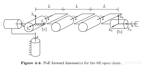
图中展示的是各关节均在零位时的状态。末端执行器的坐标系 $M$ 在零位时如下：
$$M=\left[\begin{array}{cccc}1& 0& 0& 0\\ 0& 1& 0& 3L\\ 0& 0& 1& 0\\ 0& 0& 0& 1\end{array}\right].\text{\hspace{1em}(4.15)}$$
下面对6个关节的 $w,v$ 分别描述：

1. 关节1的旋量轴方向为 $w_1=(0,0,1)$，轴1上的一点 $q_1$ 最便捷的选择的是落在固定坐标系的原点处，所以 $v_1=(0,0,0)$。
2. 关节2的旋量轴沿着固定坐标系的 $\hat{y}$ 方向，所以 $w_2=（0,1,0)$，选取 $q_2=(0,0,0)$，则 $v_2=(0,0,0)$。
3. 关节3的旋量轴方向为 $w_3=(-1,0,0)$，选取 $q_3=(0,0,0)$，则 $v_3=(0,0,0)$。
4. 关节4的旋量轴方向为 $w_4=(-1,0,0)$，选取 $q_4=(0,L,0)$，则 $v_4=(0,0,L)$。
5. 关节5的旋量轴方向为 $w_5=(-1,0,0)$，选取 $q_5=(0,2L,0)$，则 $v_5=(0,0,2L)$。
6. 关节6的旋量轴方向为 $w_6=(0,1,0)$，选取 $q_6=(0,0,0)$，则 $v_6=(0,0,0)$。

第二个公式：在末端执行器坐标系下的旋量轴

根据前述文章关于线性微分方程的一些结论中提到的，$e^{M^{-1}PM}=M^{-1}{e}^{P}M$，也可以表示成$M{e}^{M^{-1}PM}=e^{P}M$。让我们把这个结论用于式4.14，推导如下：
$$\begin{array}{rl}T(\theta )& =e^{[{\mathcal{S}}_1]{\theta }_1}\cdots e^{[{\mathcal{S}}_n]{\theta }_n}M\\ & =e^{[{\mathcal{S}}_1]{\theta }_1}\cdots M{e}^{M^{-1}[{\mathcal{S}}_n]M{\theta }_n}\\ & =e^{[{\mathcal{S}}_1]{\theta }_1}\cdots M{e}^{M^{-1}[{\mathcal{S}}_{n-1}]M{\theta }_{n-1}}{e}^{M^{-1}[{\mathcal{S}}_n]M{\theta }_n}\\ & =M{e}^{M^{-1}[{\mathcal{S}}_1]M{\theta }_1}\cdots e^{M^{-1}[{\mathcal{S}}_{n-1}]M{\theta }_{n-1}}{e}^{M^{-1}[{\mathcal{S}}_n]M{\theta }_n}\\ & =M{e}^{[{\mathcal{B}}_1]{\theta }_1}\cdots e^{[{\mathcal{B}}_{n-1}]{\theta }_{n-1}}{e}^{[{\mathcal{B}}_n]{\theta }_n}\end{array}\text{\hspace{1em}(4.16)}$$
其中，$[{\mathcal{B}}_i]=M^{-1}[{\mathcal{S}}_i]M$，如 $[{\mathcal{B}}_i]=[A{d}_{M^{-1}}]{\mathcal{S}}_i$。
式（4.16）是指数公式的另一种表示方法，其每个关节的旋量轴的表达均是在零位状态下的末端坐标系的表示。可参考上述例子进行此种方式的求解。

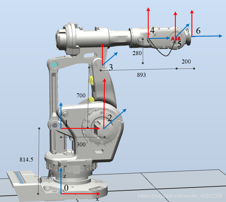
实例演示

考虑如下图所示的ABB机器人，各参数也已经标示。这里仅以固定坐标系下的运算为例，末端执行器的运算类似。

from py.core import *

if __name__ == '__main__':

    w1 = np.array([0, 0, 1])
    q1 = np.array([0, 0, 814.5])
    v1 = -np.cross(w1, q1)
    s1 = np.append(w1, v1)

    w2 = np.array([0, 1, 0])
    q2 = np.array([300, 0, 814.5])
    v2 = -np.cross(w2, q2)
    s2 = np.append(w2, v2)

    w3 = np.array([0, 1, 0])
    q3 = np.array([300, 0, 1514.5])
    v3 = -np.cross(w3, q3)
    s3 = np.append(w3, v3)

    w4 = np.array([1, 0, 0])
    q4 = np.array([1193, 0, 1794.5])
    v4 = -np.cross(w4, q4)
    s4 = np.append(w4, v4)

    w5 = np.array([0, 1, 0])
    q5 = np.array([1193, 0, 1794.5])
    v5 = -np.cross(w5, q5)
    s5 = np.append(w5, v5)

    w6 = np.array([1, 0, 0])
    q6 = np.array([1393, 0, 1794.5])
    v6 = -np.cross(w6, q6)
    s6 = np.append(w6, v6)

    M = np.array([[0, 0, 1, 1393],
                  [0, -1, 0, 0],
                  [1, 0, 0, 1794.5],
                  [0, 0, 0, 1]])
    print(M)

    S_list = np.array([s1, s2, s3, s4, s5, s6])
    print(S_list)

    theta_list = np.array(
        [np.pi / 2, np.pi / 3, np.pi / 3, np.pi / 6, np.pi / 6, np.pi / 3])

    result = FKinSpace(M, S_list.T, theta_list)
    print(result)

结果如下，4*4的变换矩阵由 (R, p)组成，代表了旋转与平移。

[[ 9.66506351e-01  5.80127019e-02 -2.50000000e-01 -5.00000000e+01]
 [-1.75240474e-01 -5.62500000e-01 -8.08012702e-01  5.40602355e+02]
 [-1.87500000e-01  8.24759526e-01 -5.33493649e-01  1.44440585e+02]
 [ 0.00000000e+00  0.00000000e+00  0.00000000e+00  1.00000000e+00]]

其中的，$FKinSpace(M,Slist.T,thetalist)$ 函数主体如下：

def IKinSpace(Slist, M, T, thetalist0, eomg, ev):
    """Computes inverse kinematics in the space frame for an open chain robot

    :param Slist: The joint screw axes in the space frame when the
                  manipulator is at the home position, in the format of a
                  matrix with axes as the columns
    :param M: The home configuration of the end-effector
    :param T: The desired end-effector configuration Tsd
    :param thetalist0: An initial guess of joint angles that are close to
                       satisfying Tsd
    :param eomg: A small positive tolerance on the end-effector orientation
                 error. The returned joint angles must give an end-effector
                 orientation error less than eomg
    :param ev: A small positive tolerance on the end-effector linear position
               error. The returned joint angles must give an end-effector
               position error less than ev
    :return thetalist: Joint angles that achieve T within the specified
                       tolerances,
    :return success: A logical value where TRUE means that the function found
                     a solution and FALSE means that it ran through the set
                     number of maximum iterations without finding a solution
                     within the tolerances eomg and ev.
    Uses an iterative Newton-Raphson root-finding method.
    The maximum number of iterations before the algorithm is terminated has
    been hardcoded in as a variable called maxiterations. It is set to 20 at
    the start of the function, but can be changed if needed.

    Example Input:
        Slist = np.array([[0, 0,  1,  4, 0,    0],
                          [0, 0,  0,  0, 1,    0],
                          [0, 0, -1, -6, 0, -0.1]]).T
        M = np.array([[-1, 0,  0, 0],
                      [ 0, 1,  0, 6],
                      [ 0, 0, -1, 2],
                      [ 0, 0,  0, 1]])
        T = np.array([[0, 1,  0,     -5],
                      [1, 0,  0,      4],
                      [0, 0, -1, 1.6858],
                      [0, 0,  0,      1]])
        thetalist0 = np.array([1.5, 2.5, 3])
        eomg = 0.01
        ev = 0.001
    Output:
        (np.array([ 1.57073783,  2.99966384,  3.1415342 ]), True)
    """
    thetalist = np.array(thetalist0).copy()
    i = 0
    maxiterations = 1000
    Tsb = FKinSpace(M, Slist, thetalist)
    Vs = np.dot(Adjoint(Tsb),
                se3ToVec(MatrixLog6(np.dot(TransInv(Tsb), T))))
    err = np.linalg.norm([Vs[0], Vs[1], Vs[2]]) > eomg \
        or np.linalg.norm([Vs[3], Vs[4], Vs[5]]) > ev
    while err and i < maxiterations:
        thetalist = thetalist \
            + np.dot(np.linalg.pinv(JacobianSpace(Slist,
                                                  thetalist)), Vs)
        i = i + 1
        Tsb = FKinSpace(M, Slist, thetalist)
        Vs = np.dot(Adjoint(Tsb),
                    se3ToVec(MatrixLog6(np.dot(TransInv(Tsb), T))))
        err = np.linalg.norm([Vs[0], Vs[1], Vs[2]]) > eomg \
            or np.linalg.norm([Vs[3], Vs[4], Vs[5]]) > ev
    return (thetalist, not err)

完整API参见Modern Robotics: Mechanics, Planning, and Control。