手写逻辑回归算法(Logistic Regression)

1、基本介绍

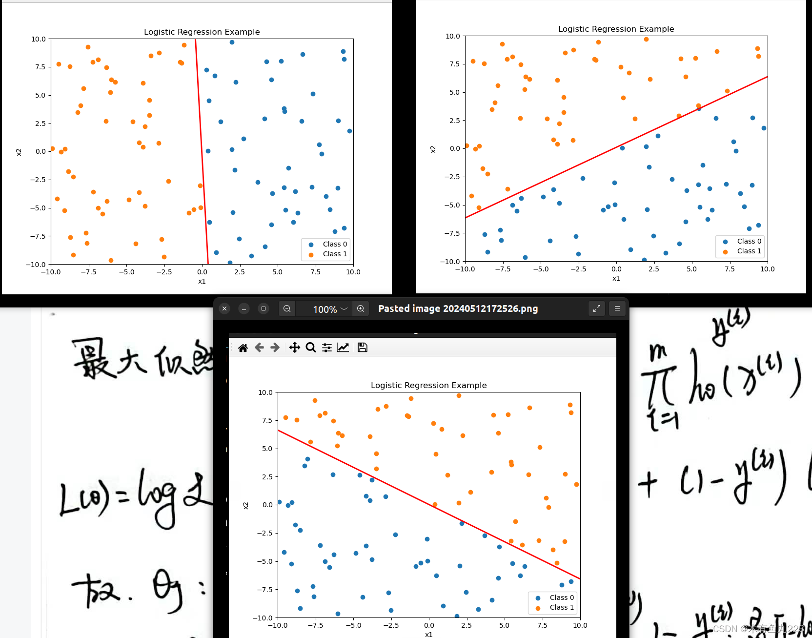
逻辑回归算法(Logistic Regression)属于判别式机器学习算法的一种，十分经典。常用来解决二分类问题。简单来说，逻辑回归就是使用sigmoid函数来建立输入特征与输出标签之间的关系。其中，我们假定输入特征$x=[x_1,x_2{]}^T,x_i\in R$，输出标签 y ∈ { 0 , 1 } y\in \{0,1\} y∈{0,1}（二分类问题）。画个图解释就是下面这样：横坐标代表特征$x_1$，纵坐标代表特征$x_2$，每一个小点就是一个样本点，蓝色代表标签值$(y=1)$，橘黄色代表标签值$(y=0)$。现在我们的任务是生成一个决策线${\theta }^{T}x=0$将两类分开。
其中，决策边界：
$${\theta }^{T}x=\left[\begin{array}{ccc}{\theta }_0& {\theta }_1& {\theta }_2\end{array}\right]\left[\begin{array}{c}1\\ x_1\\ x_2\end{array}\right]={\theta }_0+{\theta }_1{x}_1+{\theta }_2{x}_2=0\text{\hspace{1em}(1)}$$
大名鼎鼎的sigmoid函数如下，这个建立了模型输出(R)到标签概率[0,1]的映射：
$$g(x)=\frac{1}{1+e^{-x}}x\in R\text{\hspace{1em}(2)}$$
我们做如下假定，给定一个样本点的特征x，其sigmoid模型的输出作为标签为1的概率，即：
$$\begin{gathered} p(y=1|x;\theta )=h_{\theta }(x)=g({\theta }^{T}x) \\ p(y=0|x;\theta )=1-h_{\theta }(x) \end{gathered}$$
合并一下，有以下表达：
$$p(y|x;\theta )=h_{\theta }(x{)}^y.(1-h_{\theta }(x){)}^{1-y}$$
这个假定也很好理解，我们的模型训练好了参数$\theta$，采用线性的方式得到的结果带入到sigmoid函数映射到[0,1]，作为我们模型认为该点是1的概率，很合理吧，很自然吧。如果我们能够获得这么一组参数$\theta$，来了一个新的数据点(x1,x2)，我带进去一算，sigmoid的结果是0.9，那我就很高兴的预测，这个点有九成概率是1。这个思路很自然。

接下来的推导就很自然了，我们使用最大似然估计。所谓的最大似然估计，就是指我们在随机实验中，恰好拿到了我们现在已经有的这一组数据的可能性是最大的。以此标准来实现对参数$\theta$的估计。这一部分都是概率论最基本的推导。我会在原理推导部分给出详细的推导。接下来，我想叙述的是作为一个程序，我们应该如何合理的通过迭代的方式，获得比较好的参数值$\theta$。简单来说就是下面这个表达式：
$${\theta }_j:={\theta }_j+\alpha \frac{\partial }{\partial {\theta }_j}L(\theta )$$
其中，$\alpha$代表学习率，$L(\theta )$代表似然估计的值，即我们沿着使得似然估计值最大的方向上前进，经过一段时间的迭代，我们将会得到一个比较好的参数$\theta$。

2、原理推导

3、实验结果

下面是我的算法的一些结果，需要注意的是这只验证算法合理性，没有考虑停止条件，不停迭代若干次后的结果。本次实验，使用的数据是自己根据方程$y=ax1+bx2$生成的，没有任何噪声干扰。

4、代码分享

这里我提供了，数据生成代码，其生成数据并将之保存到cvs文件中。可以自己生成，也可以使用我提供的cvs文件。本人呢，python代码写得像C，大哥大姐们轻喷。就是验证一下而已。
逻辑回归算法主代码(python)：

import numpy as np
from DataGenerator import dataPlot
import pandas as pd

def cal_h_theta(theta, x):
	value = theta[0] + theta[1] * x['x1'] + theta[2] * x['x2']
	kkk = 1 / (1 + np.exp( - value))
	return kkk

if __name__ == '__main__':
	data = pd.read_csv('logistic_regression_data.csv')
	m = len(data['x1'])
	pt = dataPlot()
	pt.plotPoint(data['x1'],data['x2'], data['y'])
	theta = [0,0,0] # 初始化参数为0
	alpha = 0.01 #学习率为0.01
	
	for ii in range(1000):
		for i in range(3):
			sum_of_error = 0
			for j in range(m):
				if i == 0:
					xj = 1
				elif i == 1:
					xj = data.iloc[j]['x1']
				else:
					xj = data.iloc[j]['x2']
				sum_of_error = sum_of_error + (data.iloc[j]['y'] - cal_h_theta(theta, data.iloc[j])) * xj
		theta[i] = theta[i] + alpha * sum_of_error
	print("theta : {},{}, {}".format(theta[0], theta[1], theta[2]))
	pt.mainShow(theta[1], theta[2], theta[0])

画图程序：

import matplotlib.pyplot as plt
import os
import numpy as np

class dataPlot:
	def __init__(self):
		plt.figure(figsize=(8, 6))
	
	def mainShow(self, x1, x2, y, a, b):
		plt.clf()
		self.plotPoint(x1, x2, y)
		self.plotLine(a, b)
		plt.pause(0.1)

	def mainShow(self, a,b,c):
		plt.clf()
		self.plotPoint(self.x1, self.x2, self.y)
		self.plotLine(a, b,c)
		plt.pause(0.1)

	def plotLine(self,a,b,c):
		x1_grid = np.linspace(-10, 10, 100)
		x2_grid = np.linspace(-10, 10, 100)
		X1, X2 = np.meshgrid(x1_grid, x2_grid)
		Z = a * X1 + b * X2 + c
		plt.contour(X1, X2, Z, levels=[0], colors='r', linewidths=2)
		
	def plotPoint(self,x1, x2, y):
		self.x1 = x1
		self.x2 = x2
		self.y = y
		plt.scatter(x1[y == 0], x2[y == 0], label='Class 0')
		plt.scatter(x1[y == 1], x2[y == 1], label='Class 1')
		plt.xlabel('x1')
		plt.ylabel('x2')
		plt.title('Logistic Regression Example')
		plt.legend()
		
		figPath = "dataFig.png"
		if os.path.exists(figPath):
		os.remove(figPath)
		plt.savefig(figPath)
		def show(self):
		plt.show()

数据生成程序：

class LogisticRegressionDataGenerator:
    def __init__(self, a, b, n_samples, csv_path):
        self.a = a
        self.b = b
        self.n_samples = n_samples
        self.csv_path = csv_path
        
    def decision_boundary(self, x1, x2):
        return self.a * x1 + self.b * x2
    
    def generate_data(self):
        # 生成数据点
        np.random.seed(42)
        x1 = np.random.uniform(-10, 10, self.n_samples)
        x2 = np.random.uniform(-10, 10, self.n_samples)
        
        # 计算标签
        y = self.decision_boundary(x1, x2)
        y[y >= 0] = 1
        y[y < 0] = 0
        
        # 保存数据到CSV文件
        data = {'x1': x1, 'x2': x2, 'y': y}
        df = pd.DataFrame(data)
        df.to_csv(self.csv_path, index=False)

        return df
    def plot_data(self, x1, x2, y):
        plt.figure(figsize=(8, 6))
        plt.scatter(x1[y == 0], x2[y == 0], label='Class 0')
        plt.scatter(x1[y == 1], x2[y == 1], label='Class 1')
        
        x1_grid = np.linspace(-10, 10, 100)
        x2_grid = np.linspace(-10, 10, 100)
        X1, X2 = np.meshgrid(x1_grid, x2_grid)
        Z = self.decision_boundary(X1, X2)
        plt.contour(X1, X2, Z, levels=[0], colors='r', linewidths=2)
        
        plt.xlabel('x1')
        plt.ylabel('x2')
        plt.title('Logistic Regression Example')
        plt.legend()
        
        figPath = "dataFig.png"
        if os.path.exists(figPath):
            os.remove(figPath)
        plt.savefig(figPath)
        plt.show()


if __name__ == '__main__':
    generator = LogisticRegressionDataGenerator(a=-10, b=-0.6, n_samples=100, csv_path='logistic_regression_data.csv')
    df = generator.generate_data()

5、后续

目前，本人正在学习这块儿，尝试着自己实现一下，会比较清晰一些。虽说算法很基本，但是自己实现也能更好的体会到前人的强大以及自己的渺小。水平有限，大伙轻喷。每个帖子我会尽力把完整的代码贴出来(写得也不好)。以后呢，我打算单独整理出来一个github仓库，还没建，敬请期待。