


 博客介绍了Lumerical自动化API的多个脚本命令,如opensession、closesession等,还阐述了行波马赫 - 曾德尔调制器的多物理场仿真及结果。此外,介绍了Matlab自动化API、Python API以及Zemax接口的相关脚本命令和使用示例。
Lumerical automation API
opensession - Script command
FDTD MODE DGTD CHARGE HEAT FEEM INTERCONNECT
An interoperability command that opens a server session of selected Lumerical product via automation API. Once the session is opened, client product can call the server to execute arbitrary Lumerical script command(s) and execute them. Opened Lumerical session also allows to send and get variables from/to workspace.
| Syntax | Description |
|---|---|
| s2=opensession('device'); | When executed, this command will open a session of Device via the automation API. Accepted parameters: 'fdtd' 'mode' 'device' 'interconnect' |
Example
The following code example opens Device as a server, sends local variable 'x' to Device workspace followed by a command to manipulate the variable and the retrieves the result before closing the session:
#Opend Device session
s2=opensession('device');
#Declare local variable x
x=2;
#Send the local variable to Device workspace via API
putremotedata(s2,'x_device',x);
#Send script command to Device via API andsquare the variable
evalremote(s2,"y_device=x_device^2;");
#Get the variable from Device worksapace via API
?y=getremotedata(s2,'y_device');
#Close the session
closesession(s2);
closesession - Script command
FDTD MODE DGTD CHARGE HEAT FEEM INTERCONNECT
An interoperability command that will close an active server session of a specified Lumerical product previously opened via automation API.
| Syntax | Description |
|---|---|
| closesession(s); | Closes an active session s |
Example
The following code example opens Device as a server, sends local variable 'x' to Device workspace followed by a command to manipulate the variable and the retrieves the result before closing the session:
#Opend Device session
s2=opensession('device');
#Declare local variable x
x=2;
#Send the local variable to Device workspace via API
putremotedata(s2,'x_device',x);
#Send script command to Device via API andsquare the variable
evalremote(s2,"y_device=x_device^2;");
#Get the variable from Device worksapace via API
?y=getremotedata(s2,'y_device');
#Close the session
closesession(s2);
putremotedata - Script command
FDTD MODE DGTD CHARGE HEAT FEEM INTERCONNECT
An interoperability command that will send a variable from the client workspace into the server workspace via an active session. This works for matrices and strings (and not for structs and cell arrays).
| Syntax | Description |
|---|---|
| putremotedata(s,'y',x); | Creates variable y in the server workspace that has value of x in the client workspace via an active session s. |
Example
The following code example opens Device as a server, sends local variable 'x' to Device workspace followed by a command to manipulate the variable and the retrieves the result before closing the session:
#Opend Device session
s2=opensession('device');
#Declare local variable x
x=2;
#Send the local variable to Device workspace via API
putremotedata(s2,'x_device',x);
#Send script command to Device via API andsquare the variable
evalremote(s2,"y_device=x_device^2;");
#Get the variable from Device worksapace via API
?y=getremotedata(s2,'y_device');
#Close the session
closesession(s2);
getremotedata - Script command
FDTD MODE DGTD CHARGE HEAT FEEM INTERCONNECT
An interoperability command that will get a variable from the server workspace into the client workspace via an active session. This works for matrices and strings (and not for structs and cell arrays).
| Syntax | Description |
|---|---|
| y=getremotedata(s,'x'); | Creates variable y in the local client workspace that has value of x in the server workspace via an active session s. |
Example
The following code example opens Device as a server, sends local variable 'x' to Device workspace followed by a command to manipulate the variable and the retrieves the result before closing the session:
#Opend Device session
s2=opensession('device');
#Declare local variable x
x=2;
#Send the local variable to Device workspace via API
putremotedata(s2,'x_device',x);
#Send script command to Device via API andsquare the variable
evalremote(s2,"y_device=x_device^2;");
#Get the variable from Device worksapace via API
?y=getremotedata(s2,'y_device');
#Close the session
closesession(s2);
evalremote - Script command
FDTD MODE DGTD CHARGE HEAT FEEM INTERCONNECT
An interoperability command that will send a script commnad(s) to the server product and executes it there
| Syntax | Description |
|---|---|
| evalremote(s,"y=x^2;"); | Sends command y=x^2; to the server via an open session s and executes it |
Example
The following code example opens Device as a server, sends local variable 'x' to Device workspace followed by a command to manipulate the variable and the retrieves the result before closing the session:
#Opend Device session
s2=opensession('device');
#Declare local variable x
x=2;
#Send the local variable to Device workspace via API
putremotedata(s2,'x_device',x);
#Send script command to Device via API andsquare the variable
evalremote(s2,"y_device=x_device^2;");
#Get the variable from Device worksapace via API
?y=getremotedata(s2,'y_device');
#Close the session
closesession(s2);
Traveling Wave Mach-Zehnder Modulator
MODE CHARGE INTERCONNECT Photonic Integrated Circuits - Active
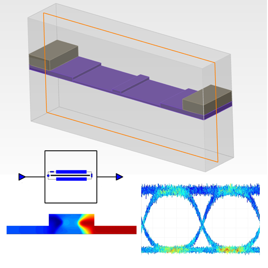
This example describes a complete multiphysics (electrical, optical, RF) simulation of a travelling wave Mach-Zehnder modulator, ending with a compact model circuit simulation in INTERCONNECT. Key results such as relative phase shift, optical transmission, transmission line bandwidth, and eye diagram are calculated.
Overview
Understand the simulation workflow and key results
This example is taken from the following publication, where a 5 mm long Si waveguide is phase modulated by a reversed bias pn junction driven by a 5mm long Al coplanar transmission line:
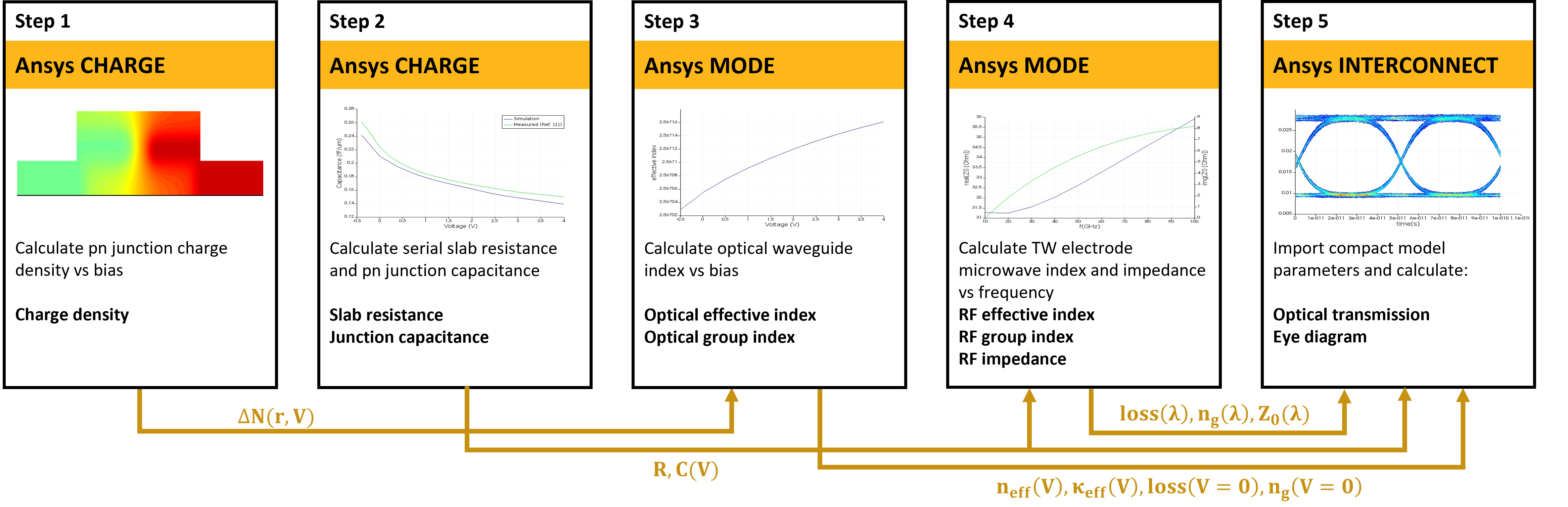
The CHARGE solver provides charge density change in the pn-junction due to changing reverse bias, along with the series slab resistance and the pn junction capacitance. The change in charge density is imported into MODE solver to calculate optical index modulation of the waveguide, while the slab resistance and junction capacitance are imported into MODE solver to calculate the RF properties of the transmission line. The optical and RF parameters, as well as the junction capacitance, are then imported into INTERCONNECT compact models to perform circuit simulation and calculate optical transmission and eye diagram.
Step 1
The CHARGE solver is first used to calculate a 2D charge density profile of the pn junction for different reverse biases. 2D simulations are much less time consuming than full 3D and in this case they are justified since the waveguide length is much larger that its thickness and width and the charge profile is relatively uniform along the waveguide. The charge density profile calculated in this step will be used in step 3 to obtain the optical refractive index modulation.
Step 2
In this step the CHARGE solver is used again to calculate the slab resistance and pn junction capacitance. The slab resistance is due to, mostly uniform, semiconductor regions that connect the transmission lines with the pn junction. As far as the pn junction itself, it can be represented just by a DC capacitance, since in reverse bias the resistance is infinite, while the capacitance is independent of the frequency. The R and C values are later imported into steps 4 (RF transmission line calculation with MODE) and 5 (circuit simulation with INTERCONNECT).
Step 3
The MODE solver is used next to calculate the optical properties of the waveguide. Based on the imported charge density vs. bias from step 1, first the change in the refractive index of the waveguide material is calculated. Then, after calculating the modes, the effective and group indices, as well as the loss, of the fundamental mode are found. These parameters are later imported into INTERCONNECT compact models. More details about the conversion of the change in charge density to the change in refractive index can be found in Additional resources .
Step 4
To calculate the RF properties of the transmission line the MODE solver is used again. In addition to defining the metallic RF co-planar transmission lines immersed in the oxide, we import the R and C values calculated in step 2, which represent a compact model of the slab and pn junction between the transmission lines. After that and similar to step 3 we find the effective and group indices and, in addition, the impedance of the fundamental mode. The parameters are found as a function of frequency, taking the voltage dependent capacitance at zero bias. These parameters will later be imported into the INTERCONNECT simulation.
Step 5
Using simulation results from previous steps, we import compact model parameters for the waveguide, optical modulator, and travelling wave electrode that make up a complete modulator circuit in INTERCONNECT. It is then possible to perform circuit simulations in both steady state and time domain to obtain an optical transmission vs. bias and frequency and an eye diagram.
Run and Results
Instructions for running the model and discussion of key results
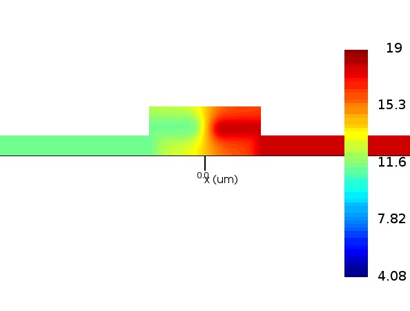
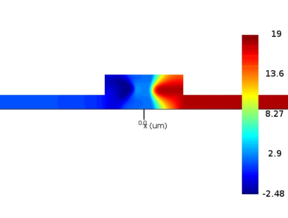
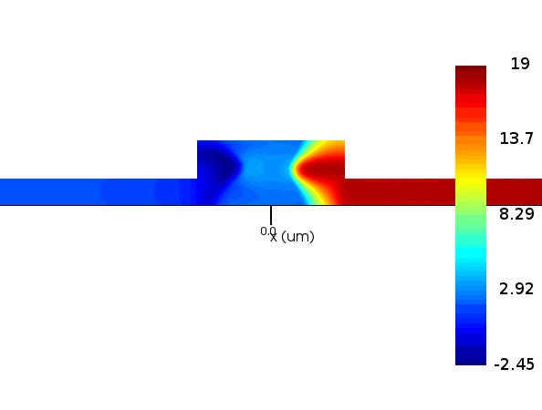
Step 1: Waveguide Charge Density vs. Bias
- Open tw_modulator_DEVICE.ldev using CHARGE.
- Run the simulation. Charge monitor "monitor_charge" is set up to save charge density in tw_modulator_charge.mat, which will later be imported into the MODE solver.
- Charge density can be visualized by selecting the CHARGE object in the objects tree, right clicking on the desired result (charge) in the result view window and visualizing it on a log scale.
The figures below show the change in charge density in the waveguide for different reverse voltages:
Step 2: Slab Resistance and pn Junction Capacitance
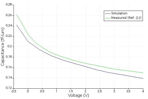
- Open tw_modulator_DEVICE_dc_C.lsf using CHARGE and run it. This script will load tw_modulator_DEVICE.ldev and calculate the DC capacitance of the pn junction using the final difference method. It will visualize the result and compare it against the publication. It will also save the voltage vs capacitance table in tw_modulator_dc_C.mat to be imported into MODE and INTERCONNECT solvers in steps 4 and 5.
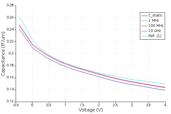
- Open tw_modulator_DEVICE_ac_RC.lsf using CHARGE and run it. This script will load tw_modulator_DEVICE.ldev and run a small signal simulation to obtain resistance and AC capacitance. It will also compare the AC capacitance with the calculated DC capacitance, confirming that the capacitance is insensitive to the frequency in reverse bias.
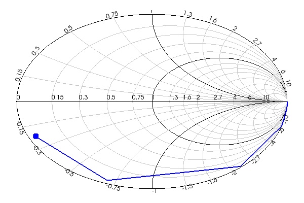
The impedance is obtained from the small signal simulation and used to derive resistance and capacitance; R and C correspond to the real and imaginary part of impedance respectively. The R value will be saved to the text file tw_modulator_Rslab_tot.dat and later used for the MODE and INTERCONNECT simulations.
The figures below show the DC capacitance and compare it to the AC capacitance and to the published result. The DC capacitance is accurate and similar to the AC capacitance as expected in the reverse bias regime. The third image is a Smith chart of the series RC circuit.
Step 3: Optical Waveguide Properties
- Open tw_modulator_optical_MODE.lms using MODE.
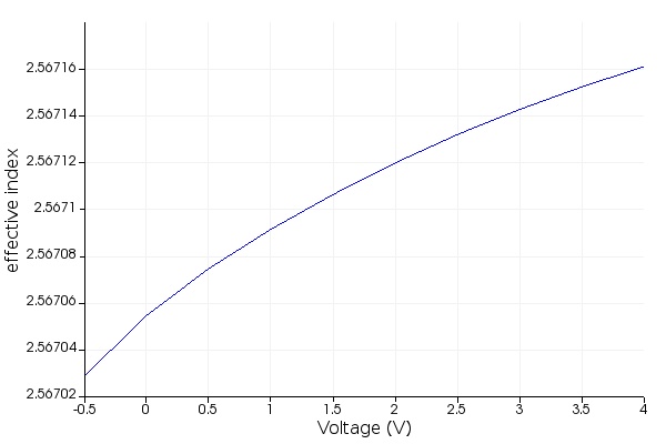
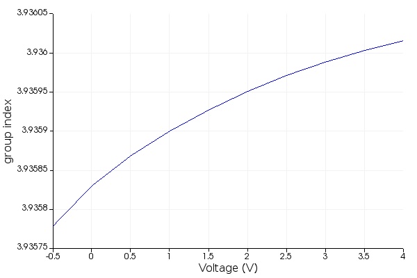
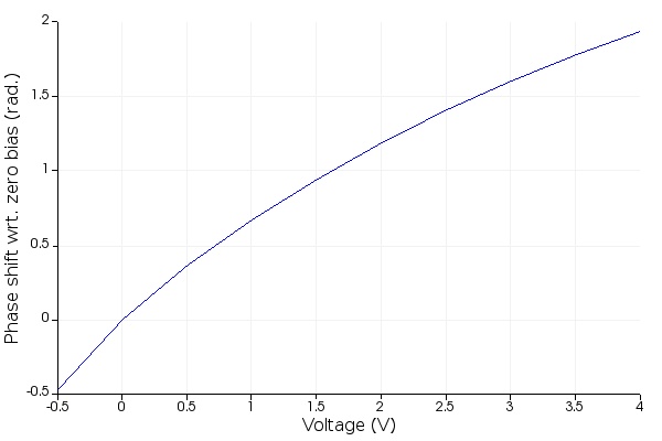
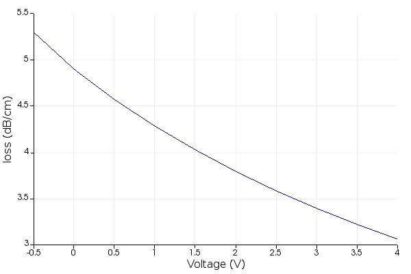
- Open script tw_modulator_optical_MODE.lsf and run it. This script will load file tw_modulator_charge.mat from step 1 into the NPDensityGridAttribute object in the object tree and calculate the optical effective and group indices of the waveguide's fundamental mode for each of the imported charge densities. It will also extract the change in the effective index with respect to the zero bias, which is the reference (middle) bias for amplitude modulation of the transmission line in INTERCONNECT. The script will also visualize the quantities of interest as shown in the figures below. The data from this step is saved into tw_modulator_optical_data.mat to be later imported into INTERCONNECT in step 5.
The figures below show the optical effective and group indices (real parts), the relative phase shift with respect to 0 V, and the loss (related to the imaginary part of the effective index).
Step 4: RF Transmission Line Properties
- Open tw_modulator_RF_MODE.lms using MODE.
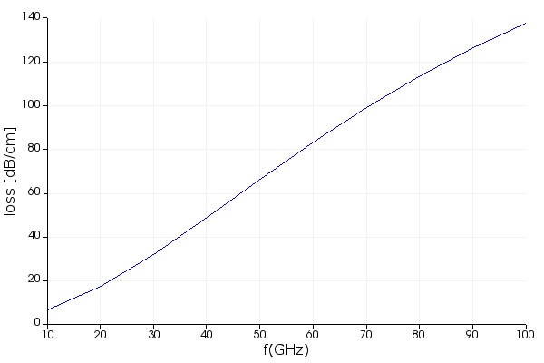
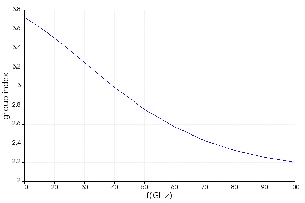
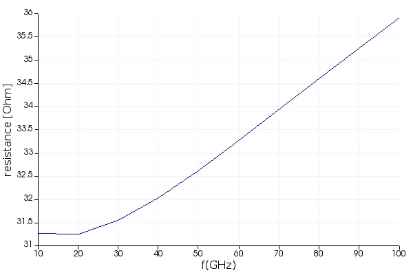
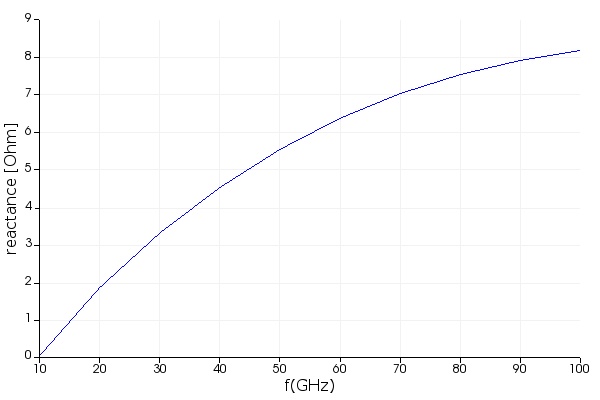
- Open script tw_modulator_RF_MODE.lsf and run it. This script will run mode analysis for frequencies between 10-100 GHz, with steps of 10 GHz, and calculate the group index, as well as the characteristic impedance and loss for the fundamental mode. It will save these parameters in tw_modulator_RF_data.mat to be imported into INTERCONNECT simulation in step 5. It will also visualize the quantities of interest as shown below.
The values of the slab resistances and pn junction capacitance (at zero bias) are copied from step 2 and set from the script. For R, the total resistance is divided by two and assigned to each region (n an p).
The figures below show the RF loss (related to the imaginary part of the RF effective index), the RF group index, and the real and imaginary parts of the characteristic impedance (resistance and reactance)
Step 5: Compact Model and Circuit Simulation
Optical Transmission With Optical Network Analyzer (ONA)
- Open file tw_modulator_INTERCONNECT_ONA.icp with INTERCONNECT, which represents the modulator photonic circuit along with an ONA measurement device. The modulator itself consists of an input waveguide Y branch followed by a waveguide and optical modulators on each branch and the output Y branch that brings the 2 modulator arms back together. The upper modulator arm has in addition a travelling wave electrode (TWE) and the phase shift is applied to this arm, while the bottom arm is kept at zero reference bias. An optical network analyzer provides the optical input to the input Y branch and receives the output optical signal from the output Y branch, while the upper arm TWE is biased with a DC signal.
- Open script tw_modulator_INTERCONNECT.lsf and run it. This script will import and set the compact model parameters obtained in steps 2-4. The waveguide elements will be set to the central frequency of 1.55 um, and the effective and group index and the loss parameters will be set at zero bias. The length of the upper arm waveguide will be set to 5 mm, while the bottom arm waveguide to 5.1 mm. The optical modulator elements will be set to the same central frequency, while the length will be set to 4.5 mm (effective phase modulation length). The change in the complex effective index vs. bias (with respect to zero bias) will also be set as a table. For the TWE, the length will be set to 5 mm and the frequency dependent tables for the loss, characteristic impedance, and group index (all at zero bias as calculated in step 4) will be loaded. The voltage dependent capacitance table will also be loaded, and the optical group index will be set to the value at zero bias. The source impedance and terminating impedance of the TWE are kept at the default value of 50 Ohm.
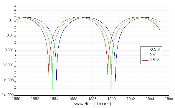
- Set the input parameter of ONA to "start and stop," "start frequency" to 1565 nm, "stop frequency" to 1550 nm, "number of points" to 1000, and "plot kind" to wavelength.
- Run 3 simulations, setting the DC output value of the DC source connected to the TWE to the values of -0.5 V, 0 V, and 0.5 V. After each simulation visualize the optical transmission from the result view of the optical network element, all on the same plot. In doing that, plot the abs^2 value of the transmission on a log plot. You can also include legend and edit the labels in the legend directly in the visualizer. The total shift in transmission is determined to be around 0.9 nm for 1 Vp-p at 0 V bias (approximately 0.8 nm in the shift of the notch can be observed in the measured data, although ripple in the data makes an accurate estimate difficult).
Eye Diagram
- Open file tw_modulator_INTERCONNECT_eye.icp with INTERCONNECT, which represents the modulator photonic circuit along with an eye diagram measurement device. The modulator circuit is the same as in step 5.1. Now, a CW laser source provides the optical input, while the upper modulator arm is driven by a pulse generator in time domain.
- Open and run script tw_modulator_INTERCONNECT.lsf to set compact model parameters (same as in step 5.1).
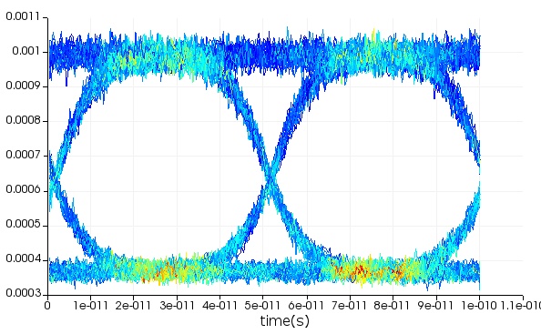
- In this simulation set the bit rate in the root element to 20 Gbits/s (this will apply to the PRBS generator and all other elements that need this information), the modulation amplitude to 1 V with the reference bias of -0.5 V in the NRZ pulse generator (signal range is then between -0.5 and 0.5 V), the laser source power to 10 mW, and the laser source wavelength to 1552.5 nm. The choice of laser power and wavelength is relatively arbitrary and in this case we chose values that give acceptable signal-to-noise ratio in the eye diagram and the eye crossing close to 50 %.
- Run the simulation. Select the eye diagram element and from the result view window visualize the eye diagram. From the same view, the extinction ratio in the eye diagram is 4.25 dB.
TWE Bandwidth With Electrical Network Analyzer (ENA)
- Open file tw_modulator_INTERCONNECT_ENA.icp with INTERCONNECT. This circuit consists of just the TWE and ENA elements. The TWE element is the same as used in previous steps.
- To set the compact model parameters of the TWE element you can run the portion of the script in tw_modulator_INTERCONNECT.lsf that applies to the TWE element (TW_1).
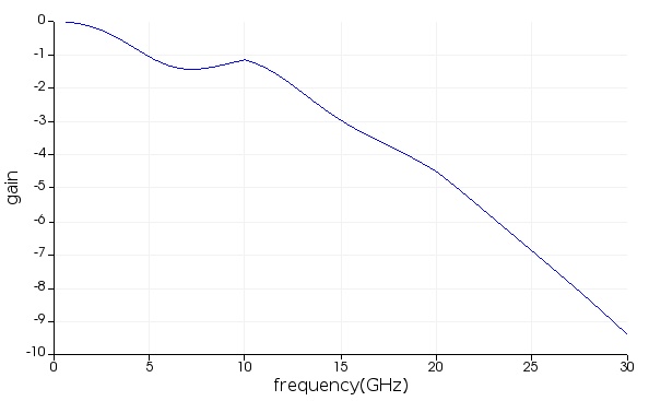
- Set the frequency range in the electrical network analyzer to 30 GHz.
- Run the simulation, and plot the gain from the ENA element. The 3 dB bandwidth is around 15 GHz.
Important Model Settings
Description of important objects and settings used in this model
Step 1: CHARGE Simulation of Charge Density
Doping Profile
The doping profile has to be modeled accurately to match the real device in order to be able to reproduce correct charge density. The user may need to fit this profile to get accurate results. One way to perform fitting is to modify doping parameters, like position and concentration, depending on which doping object was selected, until there is a good match for the pn junction capacitance. In this case the user may want to change the order of steps 1 and 2, so that step 2 is done first.
Mesh Resolution
Since the waveguide may be just a small part of the total structure (including the resistive slabs connecting the transmission lines) the mesh should be fine enough in the waveguide region to resolve the doping profile and geometry contours. Mesh size can be controlled globally in the Mesh tab of the CHARGE edit window, or by a local mesh constraint objects, in order to make the grid fine locally, while keeping it rough away from fine features to reduce simulation time.
Step 2: CHARGE Simulation of Slab Resistance and pn Junction Capacitance
DC Capacitance
When calculating DC capacitance a finite difference equation is used to find the derivative of charge density with respect to voltage. The perturbation used in finite difference should be reasonably small to get an accurate approximation of the true derivative.
AC Capacitance
For AC capacitance the ssac solver mode is used, which calculates a small signal solution on top of the DC solution at every operating point. Since the pn junction is biased in reverse mode the DC capacitance should be approximately equal to the AC capacitance. In reverse bias the parallel junction resistance is practically infinite, so there is no need to substract the resistance from total impedance before calculating capacitance.
Step 3: MODE (FDE) Simulation of the Optical Waveguide
Complex Refractive Index
Since the refractive index depends on the charge density, the charge density is imported from step 1 as a function of voltage. The theory that explains the effect of charge density on the refractive index is given at the link in Additional resources section. The charge density vs bias is imported into the 'np' object as a table and then the optical properties of the waveguide (effective and group indices) are calculated at each bias.
Fundamental Mode
Only the properties of the fundamental mode are saved and later imported into INTERCONNECT in step 5. This can be done by specifying 'mode1' string in getdata commands. To be sure the fundamental mode will be calculated set enough trial modes and set search near max index:
setanalysis('number of trial modes',10);
setanalysis('search','near n');
setanalysis('use max index',true);
Relative change in effective index: Relative change in effective index is calculated with respect to 0 V reference bias since, in subsequent circuit simulations, the pulse generator will be centered around 0 V and the reference waveguide arm will be set to 0 V.
Wavelength
Wavelength in optical mode simulations is set to 1.55 um.
Group Index
This index, which depends on the derivative of the effective index can be calculated simply by enabling an advanced option in the mode analysis with the following command
setanalysis('calculate group index',true)
Step 4: MODE (FDE) Simulation of the RF Transmission Line
RF Material Properties
RF parameters are usually not available in the database, so it may be required from the users to define their own. In this example Si is represented with a 3D conductive material with parameters: permittivity (the standard DC value taken) and conductivity (taken from the cited publication). Al transmission lines are also represented with a conductive 3D material with some reasonable values of the parameters. Since the waveguide (where the pn junction is situated) and the Si resistive slabs are much thinner than the rest of the device that comprises the co-planar transmission lines, these elements are represented with 2D rectangles with RLC material, where R values are defined for the 2 resistive slabs on both sides of the waveguide, and the waveguide is represented with a C value.
pn Junction Capacitance
This capacitance, found in step 2, is taken at 0 V, since that is the reference voltage in the circuit simulations. It is assumed that the pulse generator has a small enough amplitude so that the RF impedance and index will not change much during one cycle for a given reference bias.
Fundamental Mode
Since it is expected that the RF transmission line and the optical waveguide will have a similar propagation speed, in order to ensure the RF fundamental mode will be calculated set enough trial modes and set search near n = 4, using the following script commands:
setanalysis('number of trial modes',10);
setanalysis('search','near n');
setanalysis('use max index',false);
setanalysis('N',4);
Frequency Range
The quantities of interest, that is, loss, group index, and characteristic impedance will be calculated at the fundamental mode as a function of frequency at the reference bias 0 V. The frequency range is set from 10-100 GHz, as it is not expected that the pulse generator rates will be less than 10 Gbits/s.
Group index
Same as in step 3.
Step 5: INTERCONNECT Simulation of the Complete Modulator Circuit
Bit Rate
Random sequence of bits drives the amplitude modulation of the CW laser source. This quantity should be set at the root element, so that it can be reused in all the elements that need to know about it, which are in this case the PRBS generator and the eye diagram analyzer. To set the bit rate at these lower level elements, set their bitrate expression field to %bitrate%.
Effective Modulation Length
In the publication, not the entire length of the waveguide is doped, but only around 90%, in order to prevent current flow along the waveguide. Therefore the effective phase shift length is 4500 nm, instead of full 5000 nm. This length is used for the optical modulator elements in the two branches of the waveguide.
Waveguide and Optical Modulator
The waveguide loss and index are set at 0 V, while the relative complex index change loaded into the optical modulator is with respect to 0 V. This makes the phase shift and absorption consistent across these two connected elements.
Transmission Wave Electrode
Since only the capacitance loaded into this element can be voltage dependent, while other elements (loss, index, characteristic impedance) are just frequency dependent, they need to be calculated at a certain voltage value in step 4 and then loaded into this element. This voltage value should correspond to the reference value of 0 V as explained in the previous steps. It is assumed that these values will not change much with the changing pulse generator signal, considering relative linearity of the pn junction and Vp-p not greater than 1 V.
NRZ Pulse Generator
To make sure that the pulse generator signal is symmetric around 0 V, set the bias parameter to -0.5 V for an amplitude of 1 V. This will make sure the signal range is between -0.5 V to 0.5 V.
CW Laser Frequency and Power
These parameters are somewhat arbitrary. The power is not mentioned in the publication, nor the precise wavelength. In addition, there is a slight shift in the optical transmission curves between the simulation and publication, so the same wavelength will not work in the same way. Our choice of 10 mW and 1552.5 nm was based on having an acceptable signal-to-noise ratio in the eye diagram and an eye crossing close to 50%. This gave the extinction ratio of 4.25 dB, which is close to the value reported in the publication for 20 Gbits/s signal and 1V Vp-p.
Updating the Model With Your Parameters
Instructions for updating the model based on your device parameters
When updating the model to match your parameters, it is important to remember that multiple solvers and simulation files are involved. Changes must be made consistently in all the files. Some key parameters are listed below:
Modulator Geometry
- Length: Set new lengths of waveguide, optical modulator, and travelling wave electrode elements in step 5. Rerun step 5. Optical modulator length should be changed only if the effective phase shift length changed (doped length).
- Cross-section: Change the cross-section geometry in steps 1-4. Rerun steps 1-4 following the same instructions as the original example. Import new parameters in step 5 and rerun step 5.
Optical Source Frequency
Change the source frequency (or wavelength) in step 3 and rerun. Import new optical parameters in step 5 and set the new value of the CW laser source wavelength. Rerun step 5.
Material
- Transmission line metal: Change the transmission line material in step 4 and rerun it. Import new RF parameters into step 5 and rerun it.
- Waveguide semiconductor: Change the semiconductor material in steps 1-4. Rerun steps 1-4 following the same instructions as the original example. Import new parameters in step 5 and rerun step 5.
Doping Profile
- Shape/concentration: Change the doping profile in steps 1-2 and rerun them. Rerun steps 3-4. Import new parameters into step 5 and rerun it.
- Effective doped length: Change the length of the optical modulator elements in step 5 to correspond to the doped length. Rerun step 5.
Reference Bias
Reference bias is the bias of the lower arm of the modulator and also the mid-range value of the pulse generator output voltage. This bias was 0 V in the original example. If it is changed, but is already calculated in steps 1-2, set new capacitance in step 4 for that bias and rerun step 4. Import new RF parameters into step 5. Set new optical parameters in waveguide and TWE (just optical group index) elements in step 5. Calculate relative effective index change from step 3 with respect to the new reference voltage and load into the optical modulator elements. Rerun step 5.
Taking the Model Further
Information and tips for users that want to further customize the model
- The user may want to apply a differential drive on the upper and lower arm transmission lines in order to make the circuit more power efficient. To do this another TWE should be added to the lower arm of the modulator, which will be driven by another PRBS sequence generator followed by NRZ pulse generator. To generate a synchronized differential signal the user should set both PRBS generators to use the same seed value (non-automatic), include a digital NOT element between the PRBS and NRZ generators in the lower arm, set the bias in the NRZ generators to the same value, and the amplitudes A in the NRZ generators to the same absolute value with either the same or opposite signs, depending on what kind of differential signal is needed (e.g. (0,A,0) in the upper arm and (-A,0,-A) in the lower, or (0,A,0) in the upper and (A,0,A) in the lower). Correspondingly, when calculating the optical transmission with ONA, the appropriate voltages should be set to the upper and lower arms instead of fixing the lower arm to a constant reference value.
- If a differential drive is applied the user may want to increase the model accuracy by splitting the lower arm waveguide into a 100 um waveguide and a 5000 um waveguide and apply the modulation only to the longer waveguide.
- A more realistic model of the Y branch can be implemented by replacing it with the optical N-port S-parameter element whose parameters will be set from a separate component level simulation. More details in the Y Branch example.
Additional Resources
Additional documentation, examples and training material
Related Publications
- Tom Baehr-Jones et al., “Ultralow drive voltage silicon traveling-wave modulator”, Optics Express, Vol. 20, No. 11 (2012)
- Hao Xu et al., "Demonstration and Characterization of High-Speed Silicon Depletion-Mode Mach–Zehnder Modulators", IEEE Journal of Selected Topics in Quantum Electronics, Vol. 20, No. 4 (2014)
Matlab automation API (used in Matlab)
appopen
A MATLAB command that opens a session of selected Lumerical tool via the Matlab interoperability API. Once the session is opened, Lumerical can be called from Matlab to execute Lumerical script command(s) and execute them. Opened Lumerical session also allows Matlab to get variables from Lumerical workspace.
FDTD STACK MODE DGTD CHARGE HEAT FEEM INTERCONNECT
| Syntax | Description |
|---|---|
| h=appopen(tool, option); | When executed in Matlab, this command will open a session of FDTD via the interoperability API. Accepted tool parameters: 'fdtd' 'mode' 'device' 'interconnect' Accepted option parameter (optional): '-hide': runs the interoperability in non-graphical mode |
Example
The following Matlab code example opens FDTD session, loads an existing simulation file "MySimulation.fsp", runs the simulation, retrieves transmission from the monitor into Matlab workspace and closes FDTD.
Step 1 (only in 2020R2): Before launching MATLAB set the path; in powershell/cmd set PATH=C:\Program Files\Lumerical\v202\bin;%PATH%
Step 2:
%add Lumerical API path to Matlab; path(path,'C:\Program Files\Lumerical\FDTD\api\matlab');
appclose - Script command
FDTD MODE DGTD CHARGE HEAT FEEM INTERCONNECT
A MATLAB command that will close an active Lumerical session opened via Matlab interoperability API.
| Syntax | Description |
|---|---|
| appclose(h); | Closes an active session h |
Example
The following Matlab code example opens FDTD as a client, loads an existing simulation file "MySimulation.fsp", runs the simulation, retrieves transmission from the monitor into Matlab workspace and closes FDTD.
path(path,'C:\Program Files\Lumerical\FDTD\api\matlab');  %add Lumerical API path to Matlab;
h=appopen('fdtd');
appevalscript(h,'load("MySimulation.fsp");');
appevalscript(h,'run;');
appevalscript(h,'T=transmission("monitor");');
appevalscript(h,'T=T.T;');
x=appgetvar(h,'T');
appclose(h);
appevalscript - Script command
FDTD MODE DGTD CHARGE HEAT FEEM INTERCONNECT
A Matlab command that will execute Lumerical script command(s) in an active Lumerical session opened via Matlab interoperability API.
| Syntax | Description |
|---|---|
| appevalscript(h,'scriptcommand'); | Executes an arbitrary Lumerical script command in an active session h |
Example
The following Matlab code example opens FDTD as a client, loads an existing simulation file "MySimulation.fsp", runs the simulation, retrieves transmission from the monitor into Matlab workspace and closes FDTD.
path(path,'C:\Program Files\Lumerical\2020a\api\matlab');  %add Lumerical API path to Matlab;
h=appopen('fdtd');
appevalscript(h,'load("MySimulation.fsp");');
appevalscript(h,'run;');
appevalscript(h,'T=transmission("monitor");');
appevalscript(h,'T=T.T;');
x=appgetvar(h,'T');
appclose(h);
appgetvar - Script command
FDTD MODE DGTD CHARGE HEAT FEEM INTERCONNECT
A Matlab command that will retrieve a variable from Lumerical workspace into Matlab workspace via Matlab interoperability API.
| Syntax | Description |
|---|---|
| x=appgetvar(h,'T'); | Retrieves variable T from Lumerical workspace via an active session h and adds it into Matlab workspace as variable x |
Example
The following Matlab code example opens FDTD as a client, loads an existing simulation file "MySimulation.fsp", runs the simulation, retrieves transmission from the monitor into Matlab workspace and closes FDTD.
path(path,'C:\Program Files\Lumerical\FDTD\api\matlab');  %add Lumerical API path to Matlab;
h=appopen('fdtd');
appevalscript(h,'load("MySimulation.fsp");');
appevalscript(h,'run;');
appevalscript(h,'T=transmission("monitor");');
appevalscript(h,'T=T.T;');
x=appgetvar(h,'T');
appclose(h);
appputvar - Script command
FDTD MODE DGTD CHARGE HEAT FEEM INTERCONNECT
A Matlab command that will send a variable from Matlab workspace into Lumerical workspace via Matlab interoperability API.
| Syntax | Description |
|---|---|
| appputvar(h,'T',T_value); | Sends variable T_value from Matlab workspace via an active session h into Lumerical's workspace as variable T |
Example
The following Matlab code example opens FDTD as a client and sends/retrieves a variable to/from Lumerical FDTD workspace:
path(path,'C:\Program Files\Lumerical\FDTD\api\matlab');  %add Lumerical API path to Matlab;
h=appopen('fdtd');
a=4;
appputvar(h,'x',a);
appevalscript(h,'y=x^2;');
b=appgetvar(h,'y');

appclose(h);
Grating coupler - Matlab-driven optimization (2D)
FDTD Gratings Photonic Integrated Circuits - Passive
In this example, we will demonstrate how MATLAB can be used to drive a multi-variable nonlinear optimization of a grating coupler in FDTD via Lumerical's Automation API. In addition, we will demonstrate how to setup a MATLAB function based on arbitrary simulation parameters to specify a nonlinear constraint for the optimization.
While we focus on a specific example of a grating coupler in FDTD, the target audience includes anyone who is interested in driving and controlling Lumerical applications directly from MATLAB.
Requirements
MATLAB with Optimization Toolbox
MATLAB API Setup and Workflow
The key component required to drive simulations from MATLAB is the automation API that comes with 2016B or newer versions of Lumerical products. To allow for correct functionality, OS must know the location of Lumerical applications. On Windows machines this setup is executed automatically during the installation process, but it might be necessary for Linux users to add the install directory of given Lumerical product to their system path as described on this page.
The second step required for smooth functionality involves telling MATLAB where to look for the API before using any interoperability related commands. The MATLAB API is located in the Lumerical installation folder. In our example when we use FDTD on a Windows machine this would be typically under the following location:
C:\Program Files\Lumerical\FDTD\api\matlab
One option is to run the following command every time after MATLAB is launched and prior to using API related commands:
path(path,'C:\Program Files\Lumerical\FDTD\api\matlab');
The other, more convenient option is to add the path permanently to the startup.m file that is loaded every time MATLAB is launched.
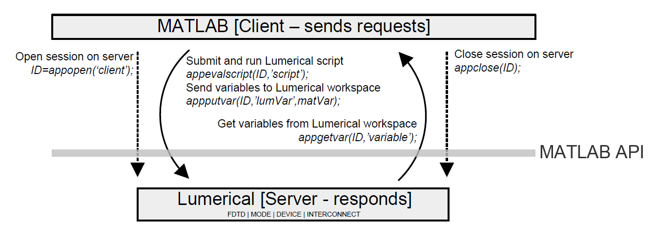
Once the MATLAB API setup is completed we can use the related interoperability commands referenced in the "See Also" section. The basic API workflow is depicted in figure 1 and it consists of four operations:
- Open one or more Lumerical session
- Send and execute Lumerical script commands to one of the active sessions
- Transfer variables between the Lumerical and the MATLAB workspace via an active session
- Close Lumerical session
Note that operations 2,3 and 4 can be executed only by referencing to an active session otherwise they will result in an error. The session referencing is done by using an unique ID that is assigned to each session during its initiation. This ID system allows the users to open and control multiple sessions at the same time.
Optimization Project Goal
For this optimization project we use the FDTD simulation file from the Grating Coupler 2D-FDTD example referenced above. This will allow us to compare the results from the MATLAB optimization with the results obtained by using a combination of Lumerical's built-in parameter sweep and particle swarm optimization utility. The goal of the optimization is to maximize the average transmission into the SOI waveguide mode in the wavelength range of 1500nm to 1600nm.
For this example, the following four parameters are chosen as the optimization variables:
- Angle theta representing the source injection angle in respect to y axis
- Source position in respect to the grating in x direction
- Grating pitch
- Grating duty cycle
In addition, this example demonstrates how to use a nonlinear constraint function that requires a specific FDTD simulation parameter as an input in addition to the variables used for optimization. To do this, we will constrain the x position of the source (xs) so the beam axis at the surface of the grating does not extend beyond the end of the grating itself (x0). This cannot be handled by a simple boundary condition since both angle theta and x position of the source are changing during the optimization. Moreover, we will use the MATLAB API to obtain the information about the distance between the source and the surface of the grating, both being inputs to the constraint function as follows:
xs≥tan(θ)×gap
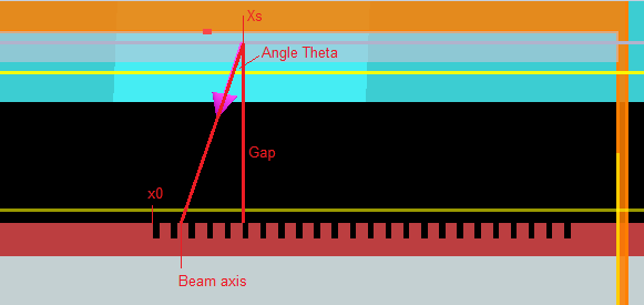
Figure 3: Visualization of the nonlinear constraint related to the source position and angle theta.
Optimization Project Setup
This project takes advantage of MATLAB "fmincon" multivariable nonlinear constrained optimization algorithm and it consists of four files:
| grating_coupler_2D_MATLAB_Optimization.fsp | 2D FDTD simulation file. This file is launched from the main MATLAB script via automation API and it returns the average transmission as a function of the input parameters provided by the optimization script |
| Coupler_Optimization_Main_Script.m | Main MATLAB script file used to:
|
| Coupler_Optimization.m | MATLAB function that is called during the optimization. It receives set of parameters from fmincon and sets up the FDTD simulation accordingly. Once the simulation is completed in FDTD, this function extracts the average transmission and passes it back to the optimization routine. Note that since fmincon searches for the global minimum, we specify the figure of merit as fval=1-T_avg; |
| confun.m | Nonlinear constraint function. Its variables are angle theta, x position of the source and the gap between the source and the grating as shown on figure 3. |
To run the example, download all three MATLAB files and the FDTD simulation file into the same folder. Open Coupler_Optimization_Main_Script.m and modify the sim_file_path to the path for the folder containing all downloaded simulation files to specify the location of the FDTD simulation file. Once the path is updated, simply run the simulation file and wait until MATLAB runs multiple optimization iterations. The final values of the optimized parameters and average transmission will be displayed in the MATLAB command window. The MATLAB script files are commented for clarity and can be reviewed in the section below:
| Note: Prior running the example, you need to update the main script for sim_file_path to reflect your folder structure |
Coupler_Optimization_Main_Script.m
clear;
%Add Lumerical Matlab API path
path(path,'C:\Program Files\Lumerical\2019b\api\matlab');
sim_file_path=('Change\This\To\Your\Folder\Structure'); % update this path to user's folder
sim_file_name=('grating_coupler_2D_Matlab_Optimization.fsp');

%Open FDTD session
h=appopen('fdtd');
%Pass the path variables to FDTD
appputvar(h,'sim_file_path',sim_file_path);
appputvar(h,'sim_file_name',sim_file_name);

%Load the FDTD simulation file and get simulation parameters
code=strcat('cd(sim_file_path);',...
    'load(sim_file_name);',...
    'select("grating_coupler_2D");',...
    'coupler_y_pos=get("y");',...
    'coupler_thickness=get("h total");',...
    'select("fiber::source");',...
    'source_y_pos=get("y");',...
    'select("fiber");',...
    'fiber_y_pos=get("y");',...
    'gap=abs(fiber_y_pos+source_y_pos-coupler_y_pos-coupler_thickness);',...
    'select("FDTD");',...
    'FDTD_span=get("x span");');
%send the script in 'code' to Lumerical FDTD
appevalscript(h,code);

%Get variables 'FDTD_span' and 'gap' from FDTD workspace to Matlab
%workspace
global gap
gap=appgetvar(h,'gap');
FDTD_span=appgetvar(h,'FDTD_span');


%Function to be optimized x(x_position,theta,pitch,dc)
f=@(x,y)Coupler_Optimization(x(1),x(2),x(3),x(4),h);

%Optimization starting points, constraints and boundaries
%The format is [x_position in um/10, theta in degrees/10, pitch in  um, duty cycle]
x0=[0.5,1.7,0.75,0.75];
A=[];
b=[];
Aeq = [];
beq=[];
lb=[0,1.1,0.5,0.5];
ub=[FDTD_span/2e-5,2,0.8,0.8];
nonlcon=@confun;

%Optimization settings
options = optimoptions('fmincon');
options = optimoptions(options,'FiniteDifferenceStepSize',1e-3);
options = optimoptions(options,'Algorithm','sqp');  %alt: interior-point
options = optimoptions(options,'MaxIter', 100);
options = optimoptions(options,'PlotFcns', { @optimplotfval });
options = optimoptions(options,'Display','iter-detailed');
options = optimoptions(options,'StepTolerance',1e-3);

%Run optimization
[x,fval]=fmincon(f,x0,A,b,Aeq,beq,lb,ub,nonlcon,options);
T_avg=1-fval;

%Display optimization results
disp(strcat({'Optimized x position: '},num2str(x(1)*10),{' um'}));
disp(strcat({'Optimized angle theta: '},num2str(x(2)*10),{' degrees'}));
disp(strcat({'Optimized pitch: '},num2str(x(3)),{' um'}));
disp(strcat({'Optimized Duty cycle: '},num2str(x(4))));
disp(strcat({'Optimized T_avg: '},num2str(T_avg)));

%Close session
appclose(h);
Coupler_Optimization.m
function y=Coupler_Optimization(x_position,theta,pitch,dc,h)

%Modify fiber position, theta, duty cycle, pitch and run the
%simulation
code=strcat('switchtolayout;',...
'select("grating_coupler_2D");',...
'set("pitch",',num2str(pitch*1e-6,16),');',...
'set("duty cycle",',num2str(dc,16),');',...
'select("fiber");',...
'set("x",',num2str(x_position*1e-5,16),');',...
'set("theta0",',num2str(theta*10,16),');',...
'run;');
appevalscript(h,code);

%Get the coupled power from T monitor to
%FDTD workspace as variable 'T_avg_FDTD'
code=strcat('T_avg_FDTD=getresult("model","T_avg");');
appevalscript(h,code);

%Get the average transmission(figure of merit) from FDTD workspace to
%MATLAB workspace
T_MATLABFun=appgetvar(h,'T_avg_FDTD');
y=1-abs(T_MATLABFun);

%Uncommnet this section to display the optimized parameters and
%figure of merit for each run in FDTD
%disp(strcat('x_pos= ',num2str(x_position,10),'...theta= ',num2str(theta,10),'...pitch= ',num2str(pitch,10),'...DC= ',num2str(dc,10)));
%disp(strcat('1-abs(T)= ',num2str(y,10)));
end
confun.m
function [c, ceq] = confun(x)

% Nonlinear inequality constraints x(x_pos,theta,pitch,dc)
global gap
c = tan(x(2)*pi/180)*gap-x(1)*1e-5;

% Nonlinear equality constraints is left empty
ceq = [];
Optimization Results
The maximum average transmission achieved with the MATLAB driven optimization is ~40%, which is in good agreement with the value obtained using the Lumerical built-in parameter sweep/particle swarm optimization routines. The optimized values for all parameters shown in table 1 are close to the reference example demonstrating that we are able to reliably find the optimal parameters using this methodology. Note that the exact values might slightly change in each optimization run as the function minimum can be achieved with a range of parameter values rather than with one exact set of values.
| Parameter | MATLAB optimization value | Reference example value |
| Theta [degrees] | 12.21 | 13.45 (fixed) |
| Source x position [um] | 3.15 | 3 um (from parameter sweep) |
| Pitch [um] | 0.6475 | 0.66 |
| Duty Cycle | 0.67 | 0.66 |
| Optimized average transmission | 0.394 | 0.388 |
Table 1: Comparison between the optimized parameters and the reference example
The time required for the four-variable optimization is comparable to the time required for the two-variable optimization with the particle swarm method, and it can be considerably influenced by setting the starting points, boundaries and the optimization parameters. Figure 4 shows comparison of two identical optimization setups that differ only in the finite difference step size (FDSS). It is clear that smaller step takes longer to estimate the trends and close in on the optimal values. As a result, we were able to achieve the optimized transmission within 8 iterations with FDSS=1e-3, while 14 iterations were required with FDSS=1e-4.
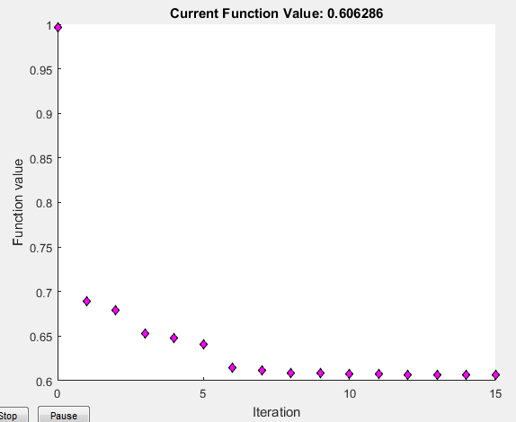
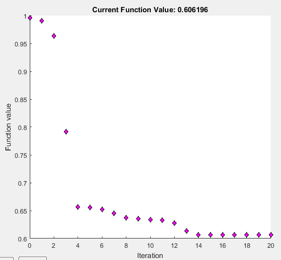
Figure 4: Tracking of the figure of merit(fval=1-Average Transmission) for different finite difference step size (left shows 1e-3 and right shows 1e-4)
Optimization tips
- If the finite difference step size is too small, the simulation result might not change significantly and the optimization algorithm might terminate prematurely. For example, in our 2D FDTD simulation, moving the source by 1nm in x direction will have minimal to no impact on the resulting average transmission.
- It is a good idea to run the optimization multiple times with slightly different starting points and boundaries to verify that the results are comparable.
- If the optimization ends with one or more parameters having the boundary value, it is likely that the minimum is artificial and the boundary should be moved.
- Sometimes it can be useful to have the optimization parameters within the same order of magnitude.
MATLAB functions (used in Lumerical)
matlabsave - Script command
FDTD MODE DGTD CHARGE HEAT FEEM INTERCONNECT
Save Lumerical workspace variables to MATLAB .mat data files.
| Syntax | Description |
|---|---|
| matlabsave(""); | Save all workspace variables to a .mat file that has the same name as the simulation file. This function does not return any data. |
| matlabsave("filename"); | Saves all workspace variables to the specified .mat file. |
| matlabsave("filename", var1, ..., varN); | Saves the specified workspace variables to the .mat file. |
Examples
Simple example:
x=1:10;
y=x^2;
matlabsave("x_squared_data", x, y);
Save data from a monitor named xy_monitor. The data is first obtained with script functions such as getdata and transmission. These workspace variables are then saved with the matlabsave function. Note that complex file names can be created with the num2str command. This is useful when doing parameter sweeps where a unique file name is required for each point in the sweep.
# get raw matrix data from the simulation
mname="xy_monitor";       # monitor name
x=getdata(mname,"x");      # position vectors associated with Ex fields
y=getdata(mname,"y");      # position vectors associated with Ex fields
Ex=getdata(mname,"Ex");     # Ex fields at monitor
T=transmission(mname);     # Power transmission through monitor

# save matrix variables x, y, Ex, T and i to a data file
i=1;
filename="results_"+num2str(i); # set filename. i could be a loop counter variable.
matlabsave(filename, x,y,Ex,T,i);
Save a Lumerical dataset (eg. Electric field vs x,y,z,f) to a .mat file. Lumerical datasets will be imported into Matlab using the struct data type.
# get electric field dataset from the simulation
mname="xy_monitor";       # monitor name
E=getresult(mname,"E");     # E fields at monitor

# save dataset to mat file
filename="ElectricField";
matlabsave(filename, E);
matlabsavelegacy - Script command
FDTD MODE DGTD CHARGE HEAT FEEM INTERCONNECT
Save workspace data to Matlab .mat data using a legacy Matlab file format required for Matlab version 7.2 and earlier. This file format does not support matrices larger than 2GB.
The command syntax is the same as the standard matlabsave command. See matlabsave for details.
matlab - Script command
FDTD MODE DGTD CHARGE HEAT FEEM INTERCONNECT
Runs a MATLAB command from the Lumerical script prompt. This gives access to extended mathematical and visualization functionality from the Lumerical script environment. If the MATLAB script integration is not enabled, this function will return an error.
The first time a MATLAB function (matlab, matlabget or matlabput) is called, a MATLAB session will be started and a connection will be established with the Lumerical scripting environment. Once this connection is established, MATLAB commands can be run using the matlab function. It is important to understand that the MATLAB and the Lumerical script variable workspaces are completely separate and independent. A MATLAB command cannot act on a variable defined in the Lumerical workspace, and vice-versa. Variables must be passed between the workspaces using the matlabget and matlabput functions. At any time you may examine the MATLAB workspace or interact with the MATLAB environment by typing commands at the MATLAB script prompt. The working directory of the MATLAB instance is always set to match the working directory of the Lumerical application.
The output from the MATLAB commands will be printed at the Lumerical script prompt. One limitation of the matlab function is that no error reporting is provided to either the Lumerical script prompt or the MATLAB prompt. MATLAB commands should be tested by typing them directly into the MATLAB prompt before they are called from a Lumerical script. The output buffer length is roughly 1e5 characters. Additional output will be truncated.
When you have a long sequence of MATLAB commands, you may find it more convenient to save them in a MATLAB m-file. Then, you can simply call the m-file by running a single command.
| See MATLAB integration setup for installation and configuration instructions. Additional tips (particularly for plotting data in Matlab) can be found in the MATLAB section of the online help. |
| Syntax | Description |
|---|---|
| matlab("command"); | command: a string containing one or more valid MATLAB commands. |
| matlab(" command_1 command_2 "); | Multi-line strings can be used in script files to contain a block of MATLAB commands. Multi-line strings are not supported at the script command prompt. |
Examples
This example will show how to use MATLAB's "surf" command to make a surface plot of the real part of Ex. It assumes that the variables x, y, Ex are already defined in the Lumerical workspace.
matlabput(x,y,Ex);
matlab("surf(y,x,real(Ex))");
This example shows how multiple MATLAB commands can be included in a single matlab function call. A log-spaced vector is created in MATLAB, then imported into the Lumerical workspace.
matlab("
 % create a logspaced vector
 x_min = 1
 x_max = 4
 x = logspace(x_min,x_max,1000)
");
matlabget(x);
matlabget - Script command
FDTD MODE DGTD CHARGE HEAT FEEM INTERCONNECT
Copies a variable from the MATLAB workspace to the script variable workspace. The resulting variable will have the same name as the MATLAB variable, and will overwrite any existing variable with the same name. If the variable does not exist in MATLAB, the command will return an error. For more information, please see the matlab command description.
| Note: Matlab script integration must be enabled in order to use this command. For more information on how to set this up see the Matlab script integration page. |
| Syntax | Description |
|---|---|
| matlabget(var1, var2,...varN); | The arguments to this command are one or more variable names that refer to variables in the MATLAB workspace. This function does not return any data. |
Examples
See the example in the matlab function description.
matlabput - Script command
FDTD MODE DGTD CHARGE HEAT FEEM INTERCONNECT
Copies a variable from Lumerical's Script Workspace to the MATLAB workspace. The resulting variable in the MATLAB workspace will have the same name as in Lumerical, and will overwrite any existing variable with the same name. If the variable does not exist in the Lumerical workspace, the command will return an error.
For more information, please see the matlab command description.
| Syntax | Description |
|---|---|
| matlabput(var1, var2,...varN); | The arguments to this command are one or more variable names that exist in the Lumerical variable workspace. This function does not return any data. |
Examples
See the examples in the matlab function description.
matlabload - Script command
FDTD MODE DGTD CHARGE HEAT FEEM INTERCONNECT
Load Matlab .mat data into workspace
| Syntax | Description |
|---|---|
| matlabload("filename"); | Load to the workspace the data of the specified .mat file. |
Examples
This is a simple example that shows how to load to workspace from a .mat data file.
#this file has variables data1, data2, data3
matlabload("myData.mat");
?workspace;
matrices:
 data1 data2 data3
Python API (lumapi module commands)
lumapi.eval - Python API method
FDTD STACK MODE DGTD CHARGE HEAT FEEM INTERCONNECT
A Python API method that executes Lumerical script command(s) in an active Lumerical session opened via the Python API.
| Syntax | Description |
|---|---|
| lumapi.eval('line1; line2;...') | When called in Python, this function will execute the Lumerical script commands in an active Lumerical session. The lines have to be complete, and it may contain multiple lines separated by a semicolon. |
This script command can be used to assign or construct variables that will later be passed to Python. This function returns no data, but can access data that is in the Lumerical workspace. The eval() method may also be used to run Lumerical script files (lsf) in your path, or functions in your workspace. For script files in another directory consider using feval - Script command.
with lumapi.FDTD(hide = True) as fdtd:
    test = fdtd.eval('z = 1 +1i;')
    print(test)
    print('Complex number z is returned as ',type(fdtd.getv('z')),str(fdtd.getv('z')))
Returns
None
Complex number z is returned as  <class 'numpy.ndarray'> [[1.+1.j]]
| Note: Previous versions of the API employed the getevalScript() method. Although this syntax still functions it will not continue to be supported. For more information on this deprecated technique of driving Lumerical's tools from Python see the Session Management -Python API.
|
lumapi.getv - Python API method
- 3 years ago
- Updated
| Syntax | Description |
|---|---|
| py_var = lumapi.getv( 'var_name') | When executed in Python, this function will get a variable from an active Lumerical session. The variable can be a string, real/complex numbers, matrix, cell or struct. |
A quick reference guide for translated datatypes.
| Lumerical | python |
|---|---|
| String | string |
| Real | float |
| Complex | np.array |
| Matrix | np.array |
| Cell array | list |
| Struct | dictionary |
| Dataset | dictionary |
String
When getv() is executed in Python, with the name of a Lumerical string variable passed as the argument, this function will return the string value of that variable to the Python environment.
with lumapi.FDTD(hide = True) as fdtd:

    #######################
    #Strings
    Lumerical = 'Lumerical Inc'
    fdtd.putv('Lum_str',Lumerical)
    print(type(fdtd.getv('Lum_str')),str(fdtd.getv('Lum_str')))
Returns
<class 'str'> Lumerical Inc
Real Number
When getv() is executed in Python, with the name of a number lsf variable passed as the argument, this function will return the value of that variable to the python environment. Integer types are not supported in Lumerical and will be returned as type float.
 with lumapi.FDTD(hide = True) as fdtd:
    #Real Number
    n = int(5)
    fdtd.putv('num',n)
    print('Real number n is returned as ',type(fdtd.getv('num')),str(fdtd.getv('num')))
Returns
Real number n is returned as <class 'float'> 5.0
Complex Number
When getv() is executed in Python, with the name of a Lumerical complex number variable passed as the argument, this function will return a numpy array with a single element to the Python environment. Likewise passing complex numbers require that they be encapsulated in a single element array. For more information see lumapi.putv(). Alternatively one can use the lumapi.eval() method to define a complex variable.
 with lumapi.FDTD(hide = True) as fdtd:
    #Complex Numbers
    z = 1 + 1.0*1j
    Z = np.zeros((1,1),dtype=complex) + z
    fdtd.putv('Z',Z[0])
    fdtd.eval('z = 1 +1i;')
    print('Complex number Z is returned as ',type(fdtd.getv('Z')),str(fdtd.getv('Z')))
    print('Complex number z is returned as ',type(fdtd.getv('z')),str(fdtd.getv('z')))
Returns
Complex number Z is returned as  <class 'numpy.ndarray'> [[1.+1.j]]
Complex number z is returned as  <class 'numpy.ndarray'> [[1.+1.j]]
Note: the different imaginary unit conventions. In python complex numbers are initialized using ‘j’ and in Lumerical this accomplished using ‘i’.
Matrix
When getv() is executed in Python, with the name of a Lumerical matrix passed as the argument, this function will return the values of that matrix variable to the python environment as a numpy array. As we saw previously these support complex data. This can be useful when defining vectors, matrices or when calling Lumerical methods that return arrays.
 with lumapi.FDTD(hide = True) as fdtd:
    ##      Vector
    rad = np.linspace(1,11)*1e-6 #np array
    height = np.arange(1,3,0.1)*1e-6 #np array
    #Pass to Lumerical
    fdtd.putv('rad',rad)
    fdtd.putv('height',height)
    #Get from Lumerical
    rad_rt=fdtd.getv('rad')
    height_rt=fdtd.getv('height')
    print('After round trip rad is ', type(rad_rt))
    print('After round trip height is ', type(height_rt))

    ###     Matrix
    M1 = np.matrix([[0,0.5,0.3,0.4,0.5,0.6], [0,2,3,4,5,6],[0,2.2,3.5,4.4,5.5,6.5]])
    M2 = np.zeros((2,2),dtype=complex)
    #Pass to Lumerical
    fdtd.putv('M1',M1)
    fdtd.putv('M2',M2)
    #Get from Lumerical
    M1_rt=fdtd.getv('M1')
    M2_rt=fdtd.getv('M2')
    print('The matrix M is ', type(M1_rt), str(M1_rt))
    print('The np array M2 is ', type(M2_rt),  str(M2_rt))

    #       Return from Lumerical
    A = fdtd.randmatrix(2,3)
    B = fdtd.zeros(1,5)
    print('The matrix A is ', type(A),  str(A))
    print('The matrix B is ', type(B),  str(B))
Returns
After round trip rad is  <class 'numpy.ndarray'>
After round trip height is  <class 'numpy.ndarray'>
The matrix M is  <class 'numpy.ndarray'> [[0.  0.5 0.3 0.4 0.5 0.6]
 [0.  2.  3.  4.  5.  6. ]
 [0.  2.2 3.5 4.4 5.5 6.5]]
The np array M2 is  <class 'numpy.ndarray'> [[0.+0.j 0.+0.j]
 [0.+0.j 0.+0.j]]
The matrix A is  <class 'numpy.ndarray'> [[0.806134   0.99917605 0.23325807]
 [0.69062098 0.53113442 0.18275802]]
The matrix B is  <class 'numpy.ndarray'> [[0. 0. 0. 0. 0.]]
Cell array
When getv() is executed in Python, with the name of a Lumerical cell passed as the argument, this function will return the cell to the Python environment as a list.
Cell arrays are ordered and can include any type of data already mentioned above, themselves and structs. Similarly, python lists are ordered and can include numerous classes as elements. These datatypes are logically equivalent.
with lumapi.FDTD(hide = True) as fdtd:
    #Cells
    C1 = [ i for i in range(11)] #list
    C2 = [[1,2,3],[4,5,6]] #list of lists
    C3 = [C1,C2,'string', 3.59]
    #Pass to Lumerical
    fdtd.putv('C_1',C1)
    fdtd.putv('C_2',C2)
    fdtd.putv('C_3',C3)
    #Get from Lumerical
    C1_rt=fdtd.getv('C_1')
    C2_rt=fdtd.getv('C_2')
    C3_rt=fdtd.getv('C_3')
    print('The cell C1 is ', type(C1_rt),  str(C1_rt))
    print('The cell C2 is ', type(C2_rt),  str(C2_rt))
    print('The cell C3 is ', type(C3_rt),  str(C3_rt))
Returns
The cell C1 is  <class 'list'> [0.0, 1.0, 2.0, 3.0, 4.0, 5.0, 6.0, 7.0, 8.0, 9.0, 10.0]
The cell C2 is  <class 'list'> [[1.0, 2.0, 3.0], [4.0, 5.0, 6.0]]
The cell C3 is  <class 'list'> [[0.0, 1.0, 2.0, 3.0, 4.0, 5.0, 6.0, 7.0, 8.0, 9.0, 10.0], [[1.0, 2.0, 3.0], [4.0, 5.0, 6.0]], 'string', 3.59]
Struct
When getv() is executed in Python, with the name of a Lumerical struct passed as the argument, this function will return the struct to the Python environment as a dictionary.
Structures are indexed by fields, but not ordered and can include any datatype mentioned above and themselves as members. Similarly, python dictionaries are indexed by keys and can include numerous classes as elements. When getv() is executed in Python, with the name of a struct lsf variable passed as the argument, this function will return the cell to the Python environment as a list.
with lumapi.FDTD(hide = True) as fdtd:
    #Struct
    D = {'greeting' : 'Hello World',                       # String data
          'pi' : 3.14,                                     # Double data
          'm' : np.array([[1.,2.,3.],[4.,5.,6.]]),         # Matrix data
          'nested_struct' : { 'e' : 2.71 } }               # Struct
    fdtd.putv('Dict', D)
    D_rt = fdtd.getv('Dict')
    print('The dictionary D is ', type(D_rt),  str(D_rt))
Returns
The dictionary D is <class 'dict'> {'greeting': 'Hello World', 'm': array([[1., 2., 3.],
Datasets
When Lumerical datasets are returned to the Python environment they are converted into Python dictionaries. For more information see Passing data - Python API.
| Note: Previous versions of the API employed the getVar() method. Although this syntax still functions it will not continue to be supported. For more information on this deprecated technique of driving Lumericals tools from Python see the Session Management -python API.
|
lumapi.putv - Python API method
FDTD STACK MODE DGTD CHARGE HEAT FEEM INTERCONNECT Automation API
A Python function that puts a variable from the local Python environment into an active Lumerical session via the Python API.
| Syntax | Description |
|---|---|
| lumapi.putv('var_name',py_var) | When executed in Python, this function will pass a variable to an open Lumerical session. The variable can be a string, real number, matrix, list or dictionary. Returns no data. |
A quick reference guide for translated datatypes.
| Lumerical | python |
|---|---|
| String | string |
| Real | float |
| Complex | np.array |
| Matrix | np.array |
| Cell array | list |
| Struct | dictionary |
| Dataset | dictionary |
String
When putv() is executed in Python, with the name of a Lumerical variable, and a string variable passed as the arguments; a string variable with the desired name and string value is created in the Lumerical session.
with lumapi.FDTD(hide = True) as fdtd:
    #Strings
    Lumerical = 'Lumerical Inc'
    fdtd.putv('Lum_str',Lumerical)
    print(type(fdtd.getv('Lum_str')),str(fdtd.getv('Lum_str')))
Returns
<class 'str'> Lumerical Inc
Real Number
When putv() is executed in python, with the name of a Lumerical variable, and a real number passed as the arguments; a variable with the desired name and real value is created in the Lumerical session. Integer types are not supported in Lumerical and will be returned as type float.
 with lumapi.FDTD(hide = True) as fdtd:
    #Real Number
    n = int(5)
    fdtd.putv('num',n)
    print('Real number n is returned as ',type(fdtd.getv('num')),str(fdtd.getv('num')))
Returns
Real number n is returned as <class 'float'> 5.0
Complex Number
One may pass a complex numpy array to the putv() method to pass a complex number. Passing complex numbers between sessions requires that they be encapsulated in a single element array since the complex class is not supported in the API. For more information see lumapi.getv(). Alternatively one can use the lumapi.eval() method to define a complex variable.
 with lumapi.FDTD(hide = True) as fdtd:
    #Complex Numbers
    z = 1 + 1.0*1j
    Z = np.zeros((1,1),dtype=complex) + z
    fdtd.putv('Z',Z[0])
    fdtd.eval('z = 1 +1i;')
    print('Complex number Z is returned as ',type(fdtd.getv('Z')),str(fdtd.getv('Z')))
    print('Complex number z is returned as ',type(fdtd.getv('z')),str(fdtd.getv('z')))
Returns
Complex number Z is returned as  <class 'numpy.ndarray'> [[1.+1.j]]
Complex number z is returned as  <class 'numpy.ndarray'> [[1.+1.j]]
NOTE: the different imaginary unit conventions. In python complex numbers are initialized using ‘j’ and in Lumerical this accomplished using ‘i’.
Numpy array
When putv() is executed in Python, with the name of a Lumerical variable name, and a numpy array passed as the arguments; a Lumerical matrix with the desired name and values is created in the Lumerical session. As we saw previously these support complex data. This useful when defining vectors, and matrices.
 with lumapi.FDTD(hide = True) as fdtd:
    ##      Vector
    rad = np.linspace(1,11)*1e-6 #np array
    height = np.arange(1,3,0.1)*1e-6 #np array
    #Pass to Lumerical
    fdtd.putv('rad',rad)
    fdtd.putv('height',height)
    #Get from Lumerical
    rad_rt=fdtd.getv('rad')
    height_rt=fdtd.getv('height')
    print('After round trip rad is ', type(rad_rt))
    print('After round trip height is ', type(height_rt))

    ###     Matrix
    M1 = np.matrix([[0,0.5,0.3,0.4,0.5,0.6], [0,2,3,4,5,6],[0,2.2,3.5,4.4,5.5,6.5]])
    M2 = np.zeros((2,2),dtype=complex)
    #Pass to Lumerical
    fdtd.putv('M1',M1)
    fdtd.putv('M2',M2)
    #Get from Lumerical
    M1_rt=fdtd.getv('M1')
    M2_rt=fdtd.getv('M2')
    print('The matrix M is ', type(M1_rt), str(M1_rt))
    print('The np array M2 is ', type(M2_rt),  str(M2_rt))

    #       Return from Lumerical
    A = fdtd.randmatrix(2,3)
    B = fdtd.zeros(1,5)
    print('The matrix A is ', type(A),  str(A))
    print('The matrix B is ', type(B),  str(B))
Returns
After round trip rad is  <class 'numpy.ndarray'>
After round trip height is  <class 'numpy.ndarray'>
The matrix M is  <class 'numpy.ndarray'> [[0.  0.5 0.3 0.4 0.5 0.6]
 [0.  2.  3.  4.  5.  6. ]
 [0.  2.2 3.5 4.4 5.5 6.5]]
The np array M2 is  <class 'numpy.ndarray'> [[0.+0.j 0.+0.j]
 [0.+0.j 0.+0.j]]
The matrix A is  <class 'numpy.ndarray'> [[0.806134   0.99917605 0.23325807]
 [0.69062098 0.53113442 0.18275802]]
The matrix B is  <class 'numpy.ndarray'> [[0. 0. 0. 0. 0.]]
List
When putv() is executed in python, with a Lumerical variable name, and a list passed as the arguments; a Lumerical cell array with the desired name and values is created in the Lumerical session.
Cell arrays are ordered and can include any type of data already mentioned above, themselves and structs. Similarly, Python lists are ordered and can include numerous classes as elements. These datatypes are logically equivalent.
with lumapi.FDTD(hide = True) as fdtd:
    #Cells
    C1 = [ i for i in range(11)] #list
    C2 = [[1,2,3],[4,5,6]] #list of lists
    C3 = [C1,C2,'string', 3.59]
    #Pass to Lumerical
    fdtd.putv('C_1',C1)
    fdtd.putv('C_2',C2)
    fdtd.putv('C_3',C3)
    #Get from Lumerical
    C1_rt=fdtd.getv('C_1')
    C2_rt=fdtd.getv('C_2')
    C3_rt=fdtd.getv('C_3')
    print('The cell C1 is ', type(C1_rt),  str(C1_rt))
    print('The cell C2 is ', type(C2_rt),  str(C2_rt))
    print('The cell C3 is ', type(C3_rt),  str(C3_rt))
Returns
The cell C1 is  <class 'list'> [0.0, 1.0, 2.0, 3.0, 4.0, 5.0, 6.0, 7.0, 8.0, 9.0, 10.0]
The cell C2 is  <class 'list'> [[1.0, 2.0, 3.0], [4.0, 5.0, 6.0]]
The cell C3 is  <class 'list'> [[0.0, 1.0, 2.0, 3.0, 4.0, 5.0, 6.0, 7.0, 8.0, 9.0, 10.0], [[1.0, 2.0, 3.0], [4.0, 5.0, 6.0]], 'string', 3.59]
Dict
When putv() is executed in Python, with a Lumerical variable name, and a Python dictionary passed as the arguments; a Lumerical struct with the desired name and values is created in the open Lumerical session.
Structures are indexed by fields, but not ordered and can include any data type mentioned above and themselves as members. Similarly, Python dictionaries are indexed by keys and can include numerous classes as elements. When getv() is executed in Python, with the name of a struct lsf variable passed as the argument, this function will return the cell to the python environment as a list.
with lumapi.FDTD(hide = True) as fdtd:
    #Struct
    D = {'greeting' : 'Hello World',                      # String data
          'pi' : 3.14,                                     # Double data
          'm' : np.array([[1.,2.,3.],[4.,5.,6.]]), # Matrix data
          'nested_struct' : { 'e' : 2.71 } }               # Struct
    fdtd.putv('Dict', D)
    D_rt = fdtd.getv('Dict')
    print('The dictionary D is ', type(D_rt),  str(D_rt))
Returns
The dictionary D is <class 'dict'> {'greeting': 'Hello World', 'm': array([[1., 2., 3.],
Datasets
When Lumerical datasets are returned to the Python environment they are converted into Python dictionaries. For more information see Passing data - Python API.
| Note: Previous versions of the API employed the putString(), putDouble(), putMatrix(), putList(), and putStruct() methods. Although this syntax still functions it will not continue to be supported. For more information on this deprecated technique of driving Lumerical's tools from Python see the Session Management -python API.
|
Zemax Interface
zbfread - Script command
zbfread reads a Zemax zbf file and adds the data into structure array that will be available in the script workspace for further processing. The structure array will contain the following data:
• Ex, Ey, Ez, x, y, z
• frequency, wavelength, index
Note that ONLY the transverse E field components can be obtained from the zbf file. The longitudinal component is not supported by the zbf format and it is populated with zero values during the read operation.
| Syntax | Description |
|---|---|
| A = zbfread("filename.zbf"); | Reads zbf file into structure array A where: A.index is the refractive index stored in the zbf file A.beam is the dataset that contains the E field vs frequency/wavelength |
| A = zbfread("filename.zbf", axis=3); | Axis = 1,2,3 is an optional parameter to specify if the beam should be rotated to propagate along x or y axis instead of the default z axis |
Example
The following code example shows how to read zbf file data into a structure array with and without rotation of the default propagation direction.
# Create spatial distribution of E field data with Gaussian distribution
x = linspace(-5e-6,5e-6,100);
y = linspace(-6e-6,6e-6,101);
X = meshgridx(x,y);
Y = meshgridy(x,y);
Ex = exp(- (X^2+Y^2)/(2e-6)^2);
Ey = 2i*Ex;
Ez = 0*Ey;
# Create dataset and add E field and wavelength data
M = rectilineardataset("E",x,y,0);
M.addparameter("lambda",500e-9);
M.addattribute("E",Ex,Ey,Ez);
M.addattribute("scalar",3*Ex);
# Write dataset M into zbf file in with and without the optional parameters
zbfwrite("testfile.zbf",M);
# Read the structured data from zbf file without rotation(default z direction)
B = zbfread("testfile.zbf");
visualize(B.beam);
# Read the structured data from zbf file and rotate the propagation direction to y
B = zbfread("testfile.zbf",axis=2);
visualize(B.beam);
zbfwrite - Script command
Zbfwrite writes a 4D dataset into a Zemax zbf file in the current directory. Data written into the zbf file:
- Ex, Ey, Ez, x, y, z
- frequency, wavelength, index
Note: ONLY the transverse E field components are written to the zbf file. The longitudinal component is not supported by the zbf format.
| Syntax | Description |
|---|---|
| zbfwrite("filename",M); | Writes dataset M into zbf file. The dataset must include one frequency or wavelength value. If the fourth dimension is named "f" or "frequency", it will be automatically converted into wavelength. Any other name will be assumed to carry wavelength information and it will not be converted. |
| zbfwrite("filename",M,index); | The optional parameter "index" is the refractive index that will be written into zbf file. A default value of "1" is used if no "index" is provided. |
| zbfwrite("filename",M,index,"attributeName"); | atributeName is an optional parameter with default value = "". This specifies the vector or scalar attribute to write. If a scalar attribute is written, it becomes an "unpolarized" zbf file. If nothing is specified(default value =""), then it will write the first vector attribute in the dataset, or the first scalar attribute if there is no vector attribute. |
| Note: The Zemax zbf file requires the data to be saved on a uniform grid of dimensions with a power of 2 (with 2n×2m |
points). The dataset will be interpolated on a grid with n and m
| defined so the mesh step is equal to or less than the smallest mesh step in the original data. |
Example
The following code example shows how to create a dataset with correct dimensions and write it into a zbf file with various optional parameters. The last section of the code reads back the saved zbf file into the structure array and plots the field profile, index, and wavelength.
# Create spatial distribution of E field data with Gaussian distribution
x = linspace(-5e-6,5e-6,100);
y = linspace(-6e-6,6e-6,101);
X = meshgridx(x,y);
Y = meshgridy(x,y);
Ex = exp(- (X^2+Y^2)/(2e-6)^2);
Ey = 2i*Ex;
Ez = 0*Ey;

# Create dataset and add E field and wavelength data
M = rectilineardataset("E",x,y,0);
M.addparameter("lambda",500e-9);
M.addattribute("E",Ex,Ey,Ez);
M.addattribute("scalar",3*Ex);

# Visualize the dataset before writing it into zbf file
visualize(M);

# Write dataset M into zbf file in with and without the optional parameters
zbfwrite("testfile1.zbf",M);
zbfwrite("testfile2.zbf",M,1);
zbfwrite("testfile3.zbf",M,1,"E");
zbfwrite("testfile4.zbf",M,2,"scalar");

# Read back the structured data from zbf file and visualize it
B = zbfread("testfile4.zbf");
visualize(B.beam);
?B.index;
B_beam=B.beam;
?B_beam.wavelength;
zbfexport - Script command
Exports data from a frequency field or field and power monitor to Zemax *.zbf file. This command can be also used to export data from a d-card to Zemax file. The return value of this command is the origin (x, y and z coordinates) of the monitor exported to the *.zbf file.
| Syntax | Description |
|---|---|
| output = zbfexport("monitorname"); | Export data from monitorname. By default, the first frequency point is exported. This function returns the origin of the monitor exported to the *.zbf file, in the format of an array with the x, y and z coordinates of the monitor origin. |
| zbfexport("monitorname",f); | Exports the frequency point specified by the index f. |
| zbfexport("monitorname",f,"filename"); | Exports to the specified "filename" without opening the file browser window. |
| Note: The Zemax zbf file requires the data to be saved on a uniform grid of dimensions with a power of 2 (with 2n×2m |
points). The dataset will be interpolated on a grid with n and m
| defined so the mesh step is equal to or less than the smallest mesh step in the original data. |
Example #1
Export data from monitor "beam_profile" to a .zbf file for Zemax. The monitor had more than one frequency point, so we elected to export the third frequency point.
?zbfexport("beam_profile",3,"test_export.zbf");
result:
1e-07
3e-07
0
Example #2
Export data from dcard named "global_mode1" to a .zbf file for Zemax. The d-card has one frequency point, so we use f index =1.
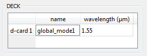
zbfexport("global_mode1",1,"testfileDcard.zbf");
zbfload - Script command
Loads data from Zemax zbf file into a d-card called "zbf_data". If "zbf_data" already exists in the deck, it will be called "zbf_data_2". After loading a zbf file with zbfload command, you can extract any of the following data:
• Ex, Ey, Ez, Hx, Hy, Hz, x, y, z
• frequency, wavelength, index
Note that the H fields are calculated during the load operation in Lumerical tools using the index from the original zbf file. Similarly, the longitudinal component in direction of propagation is not supported by the zbf format and it is populated with zero values during the load operation.
| Syntax | Description |
|---|---|
| zbfload | Select the file to load with the file browser. This function does not return any data. |
| zbfload("filename"); | Loads data from a zbf file called "filename" without a file browser. |
| zbfload("filename", propagation axis) | Loads data from a zbf file called "filename" without a file browser for a specified propagation axis. The propagation axis is an integer value that indicates the x, y and z axis. |
| zbfload("filename", propagation axis, offset); | Loads data from a zbf file called "filename" without a file browser for a specified propagation axis with the specified offset. The offset is a floating number array that indicates the x, y and z coordinates shift of the load-in data to the original data. |
Example
We have data from Zemax saved in a file named "myZemaxBeam.zbf". We use zbfload command to load the Zemax data into FDE deck for further analysis using Lumerical tools.
zbfload("myZemaxBeam.zbf");
?getdata;
 ::zbf_data
?getdata("zbf_data");
 f  wavelength  index  x  y  z  Ex  Ey  Ez
 Hx  Hy  Hz
Ex = getdata("zbf_data","Ex");
x = getdata("zbf_data","x");
y = getdata("zbf_data","y");
image(x,y,pinch(real(Ex)));
Result of zbfload operation in Eigensolver Analysis window:
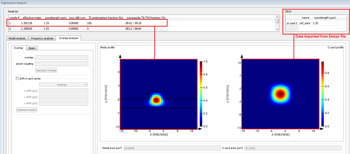
We have data from Zemax saved in a file named "myZemaxBeam.zbf". We use zbfload command to load the Zemax data twice, the first time without offset and the second time with the [x, y, z] offset as [1e-7, 3e-7, 0].
zbfload("myZemaxBeam.zbf");
Ex = getdata("zbf_data", "Ex");
x = getdata("zbf_data", "x");
y = getdata("zbf_data", "y");
image(x, y, pinch(real(Ex)));
The load in E field of zbf_data:

offset = [0.0000001, 0.0000003, 0];
zbfload("myZemaxBeam.zbf", 3, offset);
Ex = getdata("zbf_data", "Ex");
x = getdata("zbf_data", "x");
y = getdata("zbf_data", "y");
image(x, y, pinch(real(Ex)));
The load in E field of zbf_data with offset:
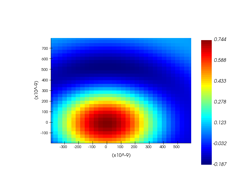


 677
677

 被折叠的 条评论
为什么被折叠?
被折叠的 条评论
为什么被折叠?
 到【灌水乐园】发言


