


switchtolayout - Script command
FDTD MODE DGTD CHARGE HEAT FEEM INTERCONNECT
Switches the solver to LAYOUT mode. The LAYOUT mode allows you to add and modify simulation objects for a new simulation. Once a simulation is run, the solver goes into ANALYSIS mode and no simulation objects can be added or modified (Except for the "Analysis" tab of analysis groups). While in ANALYSIS mode, any commands to modify objects will return errors. You must switch to LAYOUT mode before modifying any objects. Note that any available results will be lost once the solver is switched back to LAYOUT mode.
| Syntax | Description |
|---|---|
| switchtolayout; | Switches to LAYOUT mode from ANALYSIS mode. This function does not return any data. |
Example
The following script commands will first run an FDTD simulation. The solver will go to ANALYSIS mode. The "switchtolayout" command is then used to go to LAYOUT mode so that the simulation temperature can be changed in the next line.
run;
switchtolayout;
setnamed("FDTD","simulation temperature",400);   # simulation temp. set to 400 K
layoutmode - Script command
FDTD MODE DGTD CHARGE HEAT FEEM INTERCONNECT
This script command can be used to determine whether the simulation file is currently in LAYOUT mode or in ANALYSIS mode. It is important to use this command to check the status of the project file once it is opened to avoid running into an error during the subsequent operations if the file is not in the desired mode.
| Syntax | Description |
|---|---|
| ?layoutmode; | Returns 1 if in LAYOUT mode (DESIGN mode for INTERCONNECT), and 0 if in ANALYSIS mode. |
Example
The following script commands will first load a project file named "test.fsp". The aim of the script is to add a new rectangle to the existing geometry. However, if the file is in ANALYSIS mode then the "addrect" command will create an error. To avoid this, the script command "layoutmode" is first used to determine the status of the file. Then an "if/else" statement is used to add the rectangle directly if the file is already in LAYOUT mode or to add the rectangle after switching to LAYOUT mode first if the file is in ANALYSIS mode.
load("test.fsp");
status = layoutmode;

if (status == 1) {
    addrect;
}
else {
    switchtolayout;
    addrect;
}
groupscope - Script command
FDTD MODE DGTD CHARGE HEAT FEEM INTERCONNECT
Changes the group scope. Script commands that add or modify simulation object use the groupscope property to know where to act within the object tree. For example, if you want to delete everything within a particular group, set the groupscope to that group (i.e. ::model::my_group). If you want to delete all objects in the simulation, set the group scope the root level (i.e. ::model).
| Syntax | Description |
|---|---|
| ?groupscope; | returns the current group scope |
| groupscope("group_name"); | changes the group scope |
Example
Create an analysis group with a Field and Index monitor.
#create a new FDTD simulation
newproject;
addanalysisgroup;
set("name","Field_Index");
#change the group scope and add monitors to the group
groupscope("Field_Index"); # same as groupscope("::model::Field_Index");
addpower; set("name","field");
addindex; set("name","index");
selectall;
set("monitor type","3D");
set("spatial interpolation","nearest mesh cell");
set("x",0); set("y",0); set("z",0);
set("x span",1e-6); set("y span",1e-6); set("z span",1e-6);
# change the group scope back the the model
groupscope("::model");
# make a copy of the box
select("Field_Index");
copy(2e-6,0,0);
addgroup - Script command
FDTD MODE DGTD CHARGE HEAT FEEM
Adds a container group to the simulation environment. Container groups can be used to put multiple structures, monitors, and/or sources together in a single group in the objects tree. In Finite Element IDE container groups are always children of the solver regions and cannot contain any structure. If multiple solver regions are present in the Finite Element IDE objects tree then this command will add a container group to the solver region that is currently selected.
| Syntax | Description |
|---|---|
| addgroup; | Adds a container group to the simulation environment. In Finite Element IDE it will add a container group to the solver region that is currently selected. This function does not return any data. |
Example
Add a container group to the HEAT solver region (in Finite Element IDE) and put a uniform heat source in it.
select("HEAT");
addgroup;
set("name","test_group");
adduniformheat;
addtogroup("test_group");
NOTE: In this example script, since the uniform heat source is also a child of the HEAT solver, we do not need to specify the full path for the container group name (e.g. HEAT::test_group).
addanalysisgroup - Script command
Adds an analysis group to the simulation environment. Analysis groups are container objects that can contain any simulation object and associated script functions which can be used to create customize data analysis.
| Syntax | Description |
|---|---|
| addanalysisgroup; | Adds an analysis group to the simulation environment. This function does not return any data. |
Example
Add an analysis group and put a time monitor in it.
addanalysisgroup;
set("name","group");
addtime;
addtogroup("group");
To learn more about how to use analysis groups go to this page: Using Analysis Groups .
| Note: To add a pre-defined analysis group from the object library, use the addobject command. |
addobject - Script command
FDTD MODE DGTD CHARGE HEAT FEEM
Adds an object from the object library in FDTD and MODE. The command can also be used to return the names of all the available objects and analysis groups in the objects library.
| Syntax | Description |
|---|---|
| addobject("script_ID"); | Adds an object from the object library. This function does not return any data. |
| A = addobject; | Returns names of all the objects in the library and saves it in a cell array named "A". |
Example
Add a rounded cylinder object from the object library.
addobject("rounded_cyl");
set("name","test_cyl");
Print the name of all the available elements.
A = addobject;
L = length(A);
for (i = 1:L) {
    ?A{i};
}
addgridattribute - Script command
Adds a grid attribute object to the simulation environment.
| Syntax | Description |
|---|---|
| addgridattribute("type"); | Adds a grid attribute object to the simulation.
This function does not return any data. |
| addgridattribute("type",dataset); | Adds a grid attribute with spatially varying data.
|
| Data | Simulation object | Dataset type | Name for variables defining coordinate data | Name for variables defining actual data |
|---|---|---|---|---|
| Liquid crystal orientation (3 element unit vector) | 'lc orientation' grid attribute | Rectilinear | x, y, z | u |
| Rotation angles in radians | 'permittivity rotation' grid attribute | Rectilinear | x, y, z | theta, phi, psi |
| Unitary transform matrix (3x3 tensor) | 'matrix transform' grid attribute | Rectilinear | x, y, z | U |
| Charge density | 'np density' grid attribute | Unstructured | x, y, z, elements (see Dataset builder for more information) | n, p |
| Temperature in Kelvin | 'temperature' grid attribute | Unstructured | x, y, z, elements (see Dataset builder for more information) | N |
Example
The following script is an excerpt from LCD_twist.lsf in the Twisted Nematic LCD application example which defines a spatially varying liquid crystal.
# define x/y/z
x = 0;
y = 0;
z = linspace(0e-6,5e-6,100);
X = meshgrid3dx(x,y,z);
Y = meshgrid3dy(x,y,z);
Z = meshgrid3dz(x,y,z);
n = matrix(length(x),length(y),length(z),3);
# define the orientation function
n(1:length(x),1:length(y),1:length(z),1) = cos(Z*pi*1e5);
n(1:length(x),1:length(y),1:length(z),2) = sin(Z*pi*1e5);
n(1:length(x),1:length(y),1:length(z),3) = Z;
# create dataset containing orientation vectors and position parameters
LC=rectilineardataset("LC",x,y,z);
LC.addattribute("u",n);
# add LC import grid attribute
addgridattribute("lc orientation",LC);
setnamed("LC attribute","nz",50); # set resolution
importcsvlc - Script command
This command adds a LC grid attribute or analysis group containing a liquid crystal structure and LC grid attribute with data imported from a specified csv (comma separated value) file without using the GUI import wizard. The arguments allow you to make the same choices that are available in the GUI. For more information about the GUI import wizard, see Import object - Liquid crystal from CSV.
| Syntax | Description |
|---|---|
| importcsvlc(filename); | Import the csv file from the specified filename. All arguments after the filename are optional. |
| out = importcsvlc(filename,option); | Import the csv file but specify if it should be imported as a single grid attribute or added to an analysis group LC structure. |
| out = importcsvlc(filename,option,exported_from_xz_plane); | Import the csv file and specify if it was originally exported from the x-z plane. This option only applies to 2D datasets but is critical to get the orientation of the LC structure correct when it is imported into FDTD in the x-y plane. |
| out = importcsvlc(filename,option,exported_from_xz_plane,rotations); | Import the csv file with additional axis rotations. |
| Parameter | Default value | Type | Description |
|---|---|---|---|
| filename | required | string | The name of the csv file to import. May contain complete path to file, or path relative to current working directory |
| option | true | boolean | When set to 1 (true) the import will create an analysis group structure with the grid attribute and a rectangle, the same as when using the graphical import. When set to 0 (false) it will import only the grid attribute. This argument is optional |
| exported_from_xz_plane | true | boolean | Applies to 2D datasets only. This indicates that the data was originally exported from the x-z plane and this should be accounted for when it is imported into the x-y plane. |
| rotations | [0,0,0] | matrix | The optional argument allows you to specify 3 rotations around the x, y and z axes respectively that are used exactly the same way as the graphical import wizard. The matrix must have 3 elements and each value will be rounded to the nearest 90 degrees. |
Example
The following script command will import the grid attribute from file "myfile.csv" into an LC analysis group and rotate 90 degrees about the x axis.
importcsvlc("myfile.csv",true,true,[90,0,0]);
For more examples on creating LC grid attribute from script visit this kB page: LC rotation.
addport (FDTD) - Script command
Adds a port object to the ports group under the FDTD simulation region. A simulation region must be present in order to add a port. For more information about the port object see Ports . This topic addresses the addport command in FDTD - for information about the INTERCONNECT command, see addport (INTERCONNECT) .
| Syntax | Description |
|---|---|
| addport; | Adds a port. This function does not return any data. |
Example The following script adds a FDTD simulation region and port, then sets the name of the port, and selects the port modes and source mode.
addfdtd; # add FDTD simulation region
addport; # add port
# set up port
set("name","input_port");
seteigensolver("bent waveguide",true);
seteigensolver("bend radius",10e-6);
updateportmodes(1:2); # select the first 2 modes of the port
# select the second mode of the port to be the source mode
select("FDTD::ports"); # select the port group
set("source port","input_port");
set("source mode","mode 2");
addcircle - Script command
FDTD MODE DGTD CHARGE HEAT FEEM
Adds a circle primitive to the simulation environment. Circles denote physical objects which appear circular or ellipsoid from above.
| Syntax | Description |
|---|---|
| addcircle; | Adds a circle primitive to the simulation environment. This function does not return any data. |
Example
The following script commands will create a circle named "new_circle" with a radius of 5 um centered at (x,y,z) = (1, 2, 0) microns. The circle will have a thickness (z span) of 10 microns.
addcircle;
set("name","new_circle");
set("x",1e-6);
set("y",2e-6);
set("radius",5e-6);
set("z",0);
set("z span",10e-6);
addcustom - Script command
Adds a custom primitive to the simulation environment. Custom primitives are objects that are defined by equations describing the boundaries of the physical object.
| Syntax | Description |
|---|---|
| addcustom; | Adds a custom primitive to the simulation environment. This function does not return any data. |
Example
The following script commands will create a half circle with a radius of 0.5 micron in the XY plane and extrude it along the Z axis.
addcustom;
set("create 3D object by","extrusion");#  y = sqrt(0.5^2-(x-0.5)^2)
set("equation 1","sqrt("+num2str(0.5)+"^2-(x-"+num2str(0.5)+")^2)");
set("x span",1e-6);
set("y span",1e-6);
set("z span",2e-6);
The same equation can be used to create half a sphere by rotating the half circle rather than extruding it.
addcustom;
set("create 3D object by","revolution");#  y = sqrt(0.5^2-(x-0.5)^2)
set("equation 1","sqrt("+num2str(0.5)+"^2-(x-"+num2str(0.5)+")^2)");
set("x span",1e-6);
set("y span",1e-6);
set("z span",2e-6);
addimport - Script command
Adds an import primitive to the simulation environment. The import primitive can be used to create a 3D geometry by importing a surface, an image, or binary data. It can also be used to create an n,k material.
| Syntax | Description |
|---|---|
| addimport; | Adds an import primitive to the simulation environment. This function does not return any data. |
Example
The following script commands will generate a surface data and then use the data to create a layer of glass whose top surface is defined by the generated data.
# generate a surface
nx = 50;
ny = 40;
x = linspace(-6,6,nx);
y = linspace(-5,5,ny);
X = meshgridx(x,y);
Y = meshgridy(x,y);
Z = exp(-(X^2+Y^2)/4^2) * sin(pi*Y/2);
# Remember that all units are SI. We defined the surface in microns
# so all lengths must be multiplied by 1e-6
x = x*1e-6; # switch to SI units
y = y*1e-6; # switch to SI units
Z = Z*1e-6; # switch to SI units
# create substrate layer with an import object
addimport;
set("material","SiO2 (Glass) - Palik");
# upper surface and reference height
importsurface2(Z,x,y,1);
set("upper ref height",0e-6);
addpyramid - Script command
FDTD MODE DGTD CHARGE HEAT FEEM
Adds a pyramid primitive to the simulation environment.
| Syntax | Description |
|---|---|
| addpyramid; | Adds a pyramid primitive to the simulation environment. This function does not return any data. |
Example
The following script commands will add a pyramid to the simulation environment and sets its dimension
addpyramid;
set("name","my_pyramid");
set("x span bottom",5e-6);
set("x span top",3e-6);
set("y span bottom",4e-6);
set("y span top",3e-6);
set("z span",1e-6);
set("material","Si (Silicon) - Palik");
addpoly - Script command
FDTD MODE DGTD CHARGE HEAT FEEM
Adds a polygon primitive to the simulation environment. The polygon object defines a polygon in the XY plane using a set of x, y coordinates (vertices) and then extrudes it in the Z direction to create a 3D geometry.
| Syntax | Description |
|---|---|
| addpoly; | Adds a polygon primitive to the simulation environment. This function does not return any data. |
Example
The following script creates a 2D matrix to store the vertices of a polygon and uses it to create a polygon primitive.
vtx = [1,0;2,2;4,2;4,1;3,1]*1e-6;  # microns
addpoly;
set("name","random_polygon");
set("vertices",vtx);
set("z span",2e-6);
addrect - Script command
FDTD MODE DGTD CHARGE HEAT FEEM
Adds a rectangle primitive to the simulation environment.
| Syntax | Description |
|---|---|
| addrect; | Adds a rectangle primitive to the simulation environment. This function does not return any data. |
Example
The following script creates a rectangle primitive, sets its dimension, and assigns a material to it.
addrect;
set("name","new_rectangle");
set("x",1e-6);
set("x span",2e-6);
set("y",1e-6);
set("y span",5e-6);
set("z",0);
set("z span",10e-6);
set("material","Si (Silicon) - Palik");
addring - Script command
FDTD MODE DGTD CHARGE HEAT FEEM
Adds a ring primitive to the simulation environment.
| Syntax | Description |
|---|---|
| addring; | Adds a ring primitive to the simulation environment. This function does not return any data. |
Example
The following script commands will create a half-ring named "new_ring" with an inner radius of 5 um and an outer radius of 7 um centered at (x,y,z) = (1, 2, 0) microns. The ring will have a thickness (z span) of 10 microns.
addring;
set("name","new_ring");
set("x",1e-6);
set("y",2e-6);
set("inner radius",5e-6);
set("outer radius",7e-6);
set("z",0);
set("z span",10e-6);
set("theta start",0);
set("theta stop",180);
addsphere - Script command
FDTD MODE DGTD CHARGE HEAT FEEM
Adds a sphere primitive to the simulation environment.
| Syntax | Description |
|---|---|
| addsphere; | Adds a sphere primitive to the simulation environment. This function does not return any data. |
Example
The following script commands will create a sphere with a radius of 5 um centered at (x,y,z) = (1, 2, 0) microns.
addsphere;
set("name","new_sphere");
set("x",1e-6);
set("y",2e-6);
set("z",0);
set("radius",5e-6);
addsurface - Script command
Adds a surface primitive to the simulation environment.
| Syntax | Description |
|---|---|
| addsurface; | Adds primitive to the simulation environment. This function does not return any data. |
Example
Go to this KB page ( Structure - Surface ) for more details on the surface primitive and its different properties.
addstructuregroup - Script command
FDTD MODE DGTD CHARGE HEAT FEEM
Adds a structure group to the simulation environment. Structure groups are very convenient when you want to parametrize your design. You can define different parameters for the structure group and use the "setup" script to create your geometry (along with monitors and/or sources) according to those parameter values.
| Syntax | Description |
|---|---|
| addstructuregroup; | Adds a structure group to the simulation environment. This function does not return any data. |
Example
Add a structure group and put a rectangle in it.
addstructuregroup;
set("name","group");
addrect;
addtogroup("group");
Create a structure group. Add a user property named "radius" and set up the script in the structure group to add two circles to the group and set their radius to the value of the user property "radius".
addstructuregroup;
adduserprop("radius",2,0.5e-6);
myscript =      "addcircle; \n";
myscript = myscript + "copy(1e-6); \n";
myscript = myscript + "selectall; \n";
myscript = myscript + "set(\"radius\",radius);";
set("name","dimer");
set("script",myscript);
NOTE: The "myscript" string in the script above uses the escape character \n for new line and \" for double quotes within the string.
addlayer - Script command
FDTD MODE DGTD CHARGE HEAT FEEM
Adds a layer to the layer builder object. The command only works if there is a layer builder object and is selected.
| Syntax | Description |
|---|---|
| addlayer; | Adds a layer to the selected layer builder object. The name of the layer is set to "default name". This function does not return any data. |
| addlayer("name"); | Adds a layer named "name" |
Example
The following script commands will create a layer builder object and add two layers to it.
addlayerbuilder;
# Layer 1 = 100 nm layer of silver
addlayer("layer_1");
setlayer("layer_1","thickness",100e-9);
setlayer("layer_1","material","Ag (Silver) - CRC");
# Layer 2 = 500 nm layer of silicon
addlayer("layer_2");
setlayer("layer_2","thickness",500e-9);
setlayer("layer_2","material","Si (Silicon)");
addlayerbuilder - Script command
FDTD MODE DGTD CHARGE HEAT FEEM
Adds a layer builder object to the simulation environment.
| Syntax | Description |
|---|---|
| addlayerbuilder; | Adds a layer builder object to the simulation environment. This function does not return any data. |
Example
The following script commands will create a layer builder object and add two layers to it.
addlayerbuilder;
# Layer 1: 100 nm layer of silver
addlayer("layer_1");
setlayer("layer_1","thickness",100e-9);
setlayer("layer_1","pattern material","Ag (Silver) - CRC");
# Layer 2: 500 nm layer of silicon
addlayer("layer_2");
setlayer("layer_2","thickness",500e-9);
setlayer("layer_2","pattern material","Si ("Si (Silicon) - Palik");
addplanarsolid - Script command
FDTD MODE DGTD CHARGE HEAT FEEM
Adds a planar solid primitive with the specified vertices. Planar solids offer a very convenient option to create custom, complex 3D geometries. You can find more information about planar solids in this page: Structures - Planar solid.
| Syntax | Description |
|---|---|
| addplanarsolid; | Adds an empty planar solid object. |
| addplanarsolid(vtx, fct); | Adds a planer solid object whose vertices are defined by 'vtx' and whose facets are defined by 'fct' |
Example
The example below adds a planar solid cut-face box using two methods. The first method uses the facet table as a cell array and the second method uses the facet table a matrix.
method_type = 1;  # choose 1 or 2 to switch between methods
vtx = [0,0,0;
    1,0,0;
    1,1,0;
    0,1,0;
    0,0,2;
    1,0,2;
    1,1,2;
    0,1,2]*1e-6;
# Method 1: facet table as cell array
a = cell(7);
for (i = 1:7) {
 a{i} = cell(1);
}
a{1}{1} = [1,4,3,2];
a{2}{1} = [1,5,8,4];
a{3}{1} = [1,2,6,5];
a{4}{1} = [2,3,6];
a{5}{1} = [3,8,6];
a{6}{1} = [3,4,8];
a{7}{1} = [5,6,8];
if (method_type == 1) {
 addplanarsolid(vtx,a);
}
# Method 2: facet table as matrix
b = matrix(4,1,7); # max four points per polygon, max 1 polygon per facet
for (i = 1:7) {
  fpoly = a{i}{1};
  for (j = 1:length(fpoly)) {
    b(j,1,i) = fpoly(j);
    }
  }
if (method_type == 2) {
  addplanarsolid;
  set('vertices',vtx); # must be done first
  set('facets',b);
  }
stlimport - Script command
FDTD MODE DGTD CHARGE HEAT FEEM
Adds a structure to the simulation environment with structure geometry loaded from specified STL file.
| Syntax | Description |
|---|---|
| stlimport(filename,scalingFactor, vertexRadius,debugFlag); | Add a new structure from specified STL type CAD file. This function does not return any data. |
| Parameter | Default value | Type | Description | |
|---|---|---|---|---|
| filename | required | string | Name of the STL CAD file. | |
| scalingFactor | optional | 1e-6 | number | An STL file does not contain a unit. When imported to Lumerical's software, the unit is micron by default. To have the unit in nanometer, set scaling_factor 1e-9. |
| vertexRadius | optional | 1e-12 | length (in m) | Vertices may be shared by multiple triangles so the same vertex may be loaded multiple times for different triangles. The vertexRadius is the minimum distance between two vertices so that they are considered to be distinct vertices. |
| debugFlag | optional | false | boolean | If true, the following data will be printed to the script prompt: -Input Vertex Count (total number of vertices in the file) -Triangles (total number of triangles) -Filtered Vertices (number of unique vertices) -Vertex Collisions (Input Vertex Count minus Filtered Vertices) -Invalid Triangles -Expected Vertex Collisions If the number of invalid triangles is larger than 0, try adjusting the vertexRadius parameter and importing the object again. Note: If there are a large number of triangles in the STL file, the script function can take longer to run when debugFlag is set to true. |
Example
The following script commands can be used to create a 3D geometry based on the .stl file provided in this KB page: Import - STL .
filename = "stlimport_assembly.stl";
stlimport(filename);
set("material","Si (Silicon)");
stepimport - Script command
Adds a structure to the simulation environment with structure geometry loaded from specified STEP file.
| Syntax | Description |
|---|---|
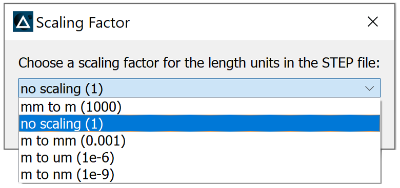
| stepimport("filename",scale_factor); | Add new structures from specified STEP (AP203/214) type CAD file. Supports multi-body parts. Only manifold solid bodies are imported - wires, surfaces, and faceted solids will not be imported. SCALE_FACTOR (optional):
|
This function does not return any data. |
| Note: How to handle the "Model size exceeds valid box" error The geometry in the finite-element IDE cannot exceed a maximum size, a fixed number of length units. This error can be avoided by changing the solver to use a larger length unit, or by supplying a smaller 'scale_factor' argument. |
Example
The following script commands can be used to create a 3D geometry based on the file provided in this KB page: Import - STEP .
filename = "stepimport.step";
stepimport(filename);
add2drect - Script command
FDTD MODE DGTD CHARGE HEAT FEEM
Adds a 2D rectangle in the simulation space.
| Syntax | Description |
|---|---|
| add2drect; | Adds a 2D rectangle in simulation space. This function does not return any data. |
| add2rect("property",value); | Adds a 2D rectangle and set its the property by specifying the "property" and value pair. |
| add2drect(struct_data); | Adds a 2D rectangle and set its the property using a struct containing "property" and value pairs. |
Example
The following script creates a 2D rectangle on the XY plane, sets its dimension, and assigns a material to it.
add2drect;
set("name","2D_rectangle");
set("surface normal",3);  # z (normal)
set("x",1e-6);
set("x span",2e-6);
set("y",1e-6);
set("y span",5e-6);
set("z",0);
set("material","Si (Silicon) - Palik");
Setting the properties while adding the object:
add2drect("name","test_obj");

# using struct
struct_data = {"name": "test_obj", "x": 1e-6};
add2drect(struct_data);
add2dpoly - Script command
FDTD MODE DGTD CHARGE HEAT FEEM
Adds a 2D polygon in the simulation space.
| Syntax | Description |
|---|---|
| add2dpoly; | Adds a 2D polygon in simulation space. This function does not return any data. |
| add2dpoly("property",value); | Adds a 2D polygon and set its the property by specifying the "property" and value pair. |
| add2dpoly(struct_data); | Adds a 2D polygon and set its the property using a struct containing "property" and value pairs. |
Example
The following script creates a 2D matrix to store the vertices of a polygon and uses it to create a 2D polygon primitive on the XY plane.
vtx = [1,0;2,2;4,2;4,1;3,1]*1e-6;  # microns
add2dpoly;
set("name","2D_polygon");
set("surface normal",3); #  1 = x (normal), 2 = y (normal), 3 = z (normal)
set("vertices",vtx);
set("z",2e-6);
Setting the properties while adding the object:
add2dpoly("name","test_obj");

# using struct
struct_data = {"name": "test_obj", "x":  1e-6};
add2dpoly(struct_data);
addwaveguide - Script command
FDTD MODE DGTD CHARGE HEAT FEEM
Adds a waveguide object in the simulation space.
| Syntax | Description |
|---|---|
| addwaveguide; | Adds a waveguide in the simulation space. This function does not return any data. |
Example
The following script commands will create a bent waveguide using 4 poles. For mode details on how the waveguide object generates the shape of the waveguide using the poles take a look at this KB page: Structures - Waveguide .
addwaveguide;

set("base width",600e-9);
set("base height",220e-9);
set("base angle",70);

pole = [0,0; 1,9; 6,9.8; 10,10]*1e-6;
set("poles",pole);

set("material","Si (Silicon) - Palik");
addeme - Script command
Adds a Eigenmode Expansion (EME) solver region to the MODE simulation environment.
| Syntax | Description |
|---|---|
| addeme; | Add an EME solver region to the simulation environment. This function does not return any data. |
Example
The following script command will add an EME solver region, set its dimension and other properties, and run the simulation. The script assumes that the simulation environment already has the geometry set up.
addeme;
# set dimension
set("x min",-8e-6);
set("y",0);
set("y span",5.5e-6);
set("z",0.5e-6);
set("z span",7e-6);
# set cell properties
set("number of cell groups",3);
set("group spans",[3e-6; 10e-6; 3e-6]);
set("cells",[1; 19; 1]);
set("subcell method",[0; 1; 0]);   # 0 = none,  1 = CVCS
# set up ports: port 1
select("EME::Ports::port_1");
set("use full simulation span",1);
set("y",0);
set("y span",5.5e-6);
set("z",0);
set("z span",7e-6);
set("mode selection","fundamental mode");
# set up ports: port 2
select("EME::Ports::port_2");
set("use full simulation span",1);
set("y",0);
set("y span",5.5e-6);
set("z",0);
set("z span",7e-6);
set("mode selection","fundamental mode");
run;
addfdtd - Script command
Adds an FDTD solver region to the simulation environment. The extent of the solver region determines the simulated volume/area in FDTD.
| Syntax | Description |
|---|---|
| addfdtd; | Adds an FDTD solver region to the simulation environment. This function does not return any data. |
Example
The following script command will add a 3D FDTD solver region, set its dimension, and run the simulation. The script assumes that the simulation environment already has the geometry and sources/monitors set up.
addfdtd;
set("dimension",2);  #  1 = 2D, 2 = 3D
set("x",0);
set("x span",2e-6);
set("y",0);
set("y span",5e-6);
set("z",0);
set("z span",10e-6);
run;
addrcwa - Script Command
Adds an RCWA solver object to the simulation environment. The extent of the solver region determines the simulated volume/area for the RCWA solver.
| Syntax | Description |
|---|---|
| addrcwa; | Adds an RCWA solver region to the simulation environment. This function does not return any data. |
Example
The following script command will add an RCWA solver region and set its dimension and size.
addrcwa;
set("simulation region", "2D Y-normal");
set("x",0);
set("x span", 1e-6);
set("z",0);
set("z span", 2e-6);
addfde - Script command
Adds a Finite Difference Eigenmode (FDE) solver region object to the MODE simulation environment.
| Syntax | Description |
|---|---|
| addfde; | Adds an FDE solver region to the simulation environment. This function does not return any data. |
Example
The following script commands will add an FDE solver region on the XY plane and calculate the eigen modes.
addfde;
set("solver type",3);
set("x",0);
set("x span",2e-6);
set("y",0);
set("y span",5e-6);
set("z",0);
findmodes;
addmesh - Script command
Adds a mesh override region to the simulation environment. The mesh override region can be used to control the size of the mesh in a certain region. In Finite Element IDE, a CHARGE solver region must be present in the objects tree for this command to work.
| Syntax | Description |
|---|---|
| addmesh; | Adds a mesh override region to the simulation environment. In Finite Element IDE, this command adds an electrical mesh which applies only to the 'CHARGE' solver. This function does not return any data. |
Example
The following script commands will add a mesh override region in FDTD, name it, set its dimension, and set the mesh constraints. The mesh object will be set to restrict the mesh in X direction only.
addmesh;
set("name","mesh_waveguide");
# set dimension
set("x",0);
set("x span",2e-6);
set("y",0);
set("y span",5e-6);
set("z",0);
set("z span",10e-6);
# enable in X direction and disable in Y,Z directions
set("override x mesh",1);
set("override y mesh",0);
set("override z mesh",0);
# restrict mesh by defining maximum step size
set("set maximum mesh step",1);
set("dx",5e-9);
addsimulationregion - Script command
Adds a simulation region to the Finite Element IDE design environment. Once created the simulation region can be linked to any existing solver.
| Syntax | Description |
|---|---|
| addsimulationregion; | Adds a simulation region to the Finite Element IDE design environment. This function does not return any data. |
Example
The following script command will add a 2D y-normal simulation region, rename it, set its dimension, and assign it to the CHARGE solver (assuming that it already exists in the objects tree).
addsimulationregion;
set("name","CHARGE simulation region");
set("dimension",2);  # 2D y-normal
set("x",0);
set("x span",2e-6);
set("y",0);
set("z",0);
set("z span",10e-6);
setnamed("CHARGE","simulation region","CHARGE simulation region");
adddevice - Script command
Adds a CHARGE solver region to the simulation environment.
| Note: The 'adddevice' command is deprecated and will be removed in future releases. Please refer to addchargesolver as a replacement. |
| Syntax | Description |
|---|---|
| adddevice; | Add a CHARGE solver region to the simulation environment. This function does not return any data. |
Example
The following script command will add a 2D y-normal CHARGE solver region, set its dimension, and run the simulation. The script assumes that the simulation environment already has the geometry and boundary conditions set up.
adddevice;
set("solver geometry",1);  #  2D y-normal
set("x",0);
set("x span",2e-6);
set("y",0);
set("z",0);
set("z span",10e-6);
run;
addvarfdtd - Script command
Adds a 2.5D varFDTD solver region to the MODE simulation environment.
| Syntax | Description |
|---|---|
| addvarfdtd; | Adds a 2.5D varFDTD simulation region. This function does not return any data. |
Example
The following script commands will add a 2.5D varFDTD solver region to the MODE simulation environment, set its dimension and simulation time, and run the simulation.
addvarfdtd;

set("x",0);
set("x span",10e-6);
set("y",0);
set("y span",10e-6);
set("z",0);
set("z span",1e-6);
set("simulation time",5000e-15);  # 5000 fs

run;
addchargesolver - Script command
Adds an electrical (CHARGE) solver region to the simulation environment.
| Syntax | Description |
|---|---|
| addchargesolver; | Adds an electrical (CHARGE) solver region to the simulation environment. This function does not return any data. |
Example
The following script command will add a 2D y-normal CHARGE solver region, set its dimension, and run the simulation. The script assumes that the simulation environment already has the geometry and boundary conditions set up.
addchargesolver;
set("solver geometry",1);  # 2D y-normal
set("x",0);
set("x span",2e-6);
set("y",0);
set("z",0);
set("z span",10e-6);
run;
addheatsolver - Script command
Adds a thermal (HEAT) solver region to the simulation environment.
| Syntax | Description |
|---|---|
| addheatsolver; | Adds a thermal (HEAT) solver region to the simulation environment. This function does not return any data. |
Example
The following script command will add a 2D y-normal HEAT solver region, set its dimension, and run the simulation. The script assumes that the simulation environment already has the geometry and boundary conditions set up.
addheatsolver;
set("solver geometry",1);  #  2D y-normal
set("x",0);
set("x span",2e-6);
set("y",0);
set("z",0);
set("z span",10e-6);
run;
addchargemesh - Script command
Adds a mesh constraint (override region) to the 'CHARGE' simulation. A CHARGE solver region must be present in the objects tree for this command to work.
| Syntax | Description |
|---|---|
| addchargemesh; | Adds a mesh constraint to the 'CHARGE' simulation environment. This function does not return any data. |
Example
The following script commands will add a mesh constraint to the CHARGE solver region in Finite Element IDE, name it, set its dimension, and set the maximum edge length for any element within the volume.
addchargesolver;
addchargemesh;
set("name","mesh_SCR");
# set dimension
set("x",0);
set("x span",2e-6);
set("y",0);
set("y span",5e-6);
set("z",0);
set("z span",10e-6);
# restrict maximum edge length for elements
set("max edge length",5e-9);
addheatmesh - Script command
Adds a mesh constraint (override region) to a 'HEAT' simulation. A HEAT solver region must be present in the objects tree for this command to work.
| Syntax | Description |
|---|---|
| addheatmesh; | Adds a mesh constraint to the 'HEAT' simulation environment. This function does not return any data. |
Example
The following script commands will add a mesh constraint to the HEAT solver region in Finite Element IDE, name it, set its dimension, and set the maximum edge length for any element within the volume.
addheatsolver;
addheatmesh;
set("name","mesh_SCR");
# set dimension
set("x",0);
set("x span",2e-6);
set("y",0);
set("y span",5e-6);
set("z",0);
set("z span",10e-6);
# restrict maximum edge length for elements
set("max edge length",5e-9);
adddgtdsolver - Script command
Adds a DGTD solver region to the simulation environment.
| Syntax | Description |
|---|---|
| adddgtdsolver; | Adds a DGTD solver region to the simulation environment. This function does not return any data. |
Example 1
The following script commands will add a DGTD solver to the objects tree and print the name of all of its properties.
adddgtdsolver;
?set;
Example 2
The following script command will add a DGTD solver region, assign it to a simulation region, and set the simulation time.
adddgtdsolver;
set("solver geometry","simulation region 1");
set("simulation time",100e-15);  # 100 fs
adddgtdmesh - Script command
Adds a mesh constraint (override region) to a 'DGTD' simulation. A DGTD solver region must be present in the objects tree for this command to work.
| Syntax | Description |
|---|---|
| adddgtdmesh; | Adds a mesh constraint to the 'DGTD' simulation environment. This function does not return any data. |
Example 1
The following script commands will add a mesh constraint to the DGTD solver already present in the objects tree and print the name of all of its properties.
adddgtdmesh;
?set;
Example 2
The following script commands will add a mesh constraint to the DGTD solver region in Finite Element IDE, name it, assign it to a specific surface between two domains, and set the maximum edge length for any element on the surface.
adddgtdsolver;
adddgtdmesh;
set("name","mesh_surface");
set("geometry type","surface");
set("surface type","domain:domain");
set("domain 1",2);
set("domain 2",3);
set("max edge length",0.05e-6);
addfeemsolver - Script command
Adds a FEEM solver region to the simulation environment.
| Syntax | Description |
|---|---|
| addfeemsolver; | Adds a FEEM solver region to the simulation environment. This function does not return any data. |
Example 1
The following script commands will add a FEEM solver to the objects tree and print the name of all of its properties.
addfeemsolver;
?set;
Example 2
The following script command will add a FEEM solver region and assign it to a simulation region.
addfeemsolver;
set("solver geometry","simulation region 1");
addfeemmesh - Script command
Adds a mesh constraint (override region) to a 'FEEM' simulation.. A FEEM solver region must be present in the objects tree for this command to work.
| Syntax | Description |
|---|---|
| addfeemmesh; | Adds a mesh constraint to the 'FEEM' simulation environment. This function does not return any data. |
Example 1
The following script commands will add a mesh constraint to the FEEM solver already present in the objects tree and print the name of all of its properties.
addfeemmesh;
?set;
Example 2
The following script commands will add a mesh constraint to the FEEM solver region in Finite Element IDE, name it, assign it to a specific surface between two domains, and set the maximum edge length for any element on the surface.
addfeemsolver;
addfeemmesh;
set("name","mesh_surface");
set("geometry type","surface");
set("surface type","domain:domain");
set("domain 1",2);
set("domain 2",3);
set("max edge length",0.05e-6);
adddipole - Script command
Adds a dipole source to the simulation environment. In MODE the command requires an active varFDTD solver region in the objects tree.
| Syntax | Description |
|---|---|
| adddipole; | Adds a dipole source to the simulation environment. This function does not return any data. |
Example
The following script commands will add a dipole source to the FDTD simulation environment and set its position.
adddipole;
set("x",0);
set("y",-1e-6);
set("z",5e-6);
addgaussian - Script command
Adds a Gaussian source to the simulation environment.
| Syntax | Description |
|---|---|
| addgaussian; | Adds a Gaussian source to the simulation environment. This function does not return any data. |
Example
The following script command will add a Gaussian source in the simulation environment that will propagate in the negative z direction. The script will set the dimension (and position) of the source and will define the beam waist radius using scalar approximation.
addgaussian;
set("injection axis","z");
set("direction","backward");
set("x",0);
set("x span",2e-6);
set("y",0);
set("y span",5e-6);
set("z",10e-6);
set("use scalar approximation",1);
set("waist radius w0",0.5e-6);
set("distance from waist",-5e-6);
addplane - Script command
Adds a plane wave source to the simulation environment.
For FDTD and MODE
| Syntax | Description |
|---|---|
| addplane; | Adds a plane wave source to the simulation environment. This function does not return any data. |
Example
The following script command will add a plane wave source in the simulation environment that will propagate in the negative z direction. The script will set the dimension (and position) of the source and will define the frequency range.
addplane;
set("injection axis","z");
set("direction","backward");
set("x",0);
set("x span",2e-6);
set("y",0);
set("y span",5e-6);
set("z",3e-6);
set("wavelength start",0.3e-6);
set("wavelength stop",1.2e-6);
For DGTD:
Adds a plane wave source to the 'DGTD' solver in Finite Element IDE. A DGTD solver region must be present in the objects tree for this command to work.
| Syntax | Description |
|---|---|
| addplane; | Adds a plane wave source to the 'DGTD' solver. This function does not return any data. |
Example 1
The following script commands will add a plane wave source to the 'DGTD' solver already present in the objects tree and print the name of all of its properties.
addplane;?set;
Example 2
The following script commands will add a plane wave source to the 'DGTD' solver, change its name, and set up its properties. The script then sets the solid named "2D rectangle" as the injection surface.
addplane;
set("name","plane_wave");# set the propagation directionset("direction definition","axis");set("direction","backward");set("angle theta",30);set("angle phi",60);
# set the polarization angleset("polarization angle",90);
# set the injection surfaceset("surface type","solid");set("solid","2D rectangle");
addmode - Script command
Adds a mode source to the simulation environment for FDTD. For MODE, adds an eigenmode (FDE) solver region to the simulation environment.
| Note: The 'addmode' command is deprecated in MODE and will be removed in future releases. Please refer to addfde as a replacement. |
| Syntax | Description |
|---|---|
| addmode; | For FDTD: Add a mode source to the simulation environment. This function does not return any data. |
| addmode; | For MODE: Add an eigenmode solver to the simulation environment. |
Example
The following script commands will add a mode source in FDTD and set its dimension and injection axis.
addmode;
set("injection axis","x");
set("x",0);
set("y",0);
set("y span",5e-6);
set("z",0);
set("z span",10e-6);
The following script commands will add an eigenmode (FDE) solver region in MODE on the XY plane and calculate the eigen modes.
addmode;
set("solver type",3);
set("x",0);
set("x span",2e-6);
set("y",0);
set("y span",5e-6);
set("z",0);
findmodes;
addmodesource - Script command
Adds a mode source to the 2.5D varFDTD simulation environment. The varFDTD solver object must be set as the active solver for this command to work.
| Syntax | Description |
|---|---|
| addmodesource; | Adds a mode source to the varFDTD solver region. This function does not return any data. |
Example
The following script commands will add a mode source to the varFDTD solver region in MODE and select the injection axis.
addmodesource;
set("injection axis","x");
set("x",0);
set("y",0);
set("y span",5e-6);
addtfsf - Script command
Adds a Total Field Scattered Field (TFSF) source to the simulation environment.
| Syntax | Description |
|---|---|
| addtfsf; | Add a total field scattered field source to the simulation environment. This function does not return any data. |
Example
The following script command will add a plane wave source in the FDTD simulation environment that will propagate in the negative z direction. The script will set the dimension (and position) of the source and will define the frequency range.
addtfsf;

set("injection axis","z");
set("direction","backward");
set("x",0);
set("x span",2e-6);
set("y",0);
set("y span",5e-6);
set("z",3e-6);
set("z span",6e-6);
set("wavelength start",0.3e-6);
set("wavelength stop",1.2e-6);
addimportedsource - Script command
Adds an imported source to the simulation environment.
| Syntax | Description |
|---|---|
| addimportedsource; | Adds an imported source to the simulation environment. This function does not return any data. |
Example
The following script commands will add an imported source to the simulation environment, assign a name to it and load an E field profile from a *.mat file.
addimportedsource;
set("name","source2");
# Load a field profile saved in Matlab file named myfile.mat
select("source2");
importdataset("myfile.mat");
To see an example of how script commands can be used to create an imported source using monitor data go to this KB page: Custom source profile from monitor data .
addindex - Script command
Adds an index monitor to the simulation environment. In MODE an active varFDTD region needs to be present for this command to work.
| Syntax | Description |
|---|---|
| addindex; | Adds an index monitor to the simulation environment. This function does not return any data. |
Example
The following script command will add a 2D y-normal index monitor to the simulation region and set its dimension.
addindex;
set("name","index_monitor");
set("monitor type",2);  # 2D y-normal
set("x",0);
set("x span",5e-6);
set("y",0);
set("z",10e-6);
set("z span",5e-6);
If an FDTD the index monitor holds results automatically without running simulations if a solver region is present. The following script command will add a solver region following the script above and will visualize the index preview.
addfdtd;
n = getresult("index_monitor","index preview");
visualize(n);
addeffectiveindex - Script command
Adds an effective index monitor to the simulation environment. This command requires the presence of an active varFDTD solver region.
| Syntax | Description |
|---|---|
| addeffectiveindex; | Adds an effective index monitor to the varFDTD solver region. This function does not return any data. |
Example
The following script command will add an effective index monitor to the simulation region and set its dimension.
addeffectiveindex;
set("name","neff");
set("x",0);
set("x span",5e-6);
set("y",0);
set("y span",5e-6);
addtime - Script command
Adds a time monitor to the simulation environment. The time monitor provides time-domain information for field components over the course of the simulation
| Syntax | Description |
|---|---|
| addtime; | Adds a time monitor to the simulation environment. This function does not return any data. |
Example
The following script command will add a point time monitor to the simulation region and set its position.
addtime;

set("name","time_1");
set("monitor type",1);  # point
set("x",0);
set("y",0);
set("z",10e-6);
addmovie - Script command
Adds a movie monitor to the simulation environment. Movie monitors capture a desired field component over the region spanned by the monitor for the duration of the simulation.
| Syntax | Description |
|---|---|
| addmovie; | Adds a movie monitor to the simulation environment. This function does not return any data. |
Example
The following script commands will add a 2D z-normal movie monitor to the simulation region, set its location and dimension, and set its resolution while keeping the aspect ratio locked. Locking the aspect ratio ensures that the video will keep the shape of the monitor data.
addmovie;
set("name","movie_1");
set("monitor type",3);  # 1 = 2D x-normal,  2 = 2D y-normal,  3 = 2D z-normal
set("x",0);
set("x span",5e-6);
set("y",0);
set("y span",5e-6);
set("z",0);
set("lock aspect ratio",1);
set("horizontal resolution",240);
addprofile - Script command
Adds a frequency domain field profile monitor to the simulation environment. Unlike the 'field and power' monitor, the 'profile' monitor does not snap to the nearest mesh cell and uses interpolation to record the data exactly where the monitor is located. This can be useful in a few situations, but the extra interpolation required can slightly reduce the accuracy of the data. In most situations, we recommend using the 'field and power' monitor.
| Syntax | Description |
|---|---|
| addprofile; | Adds a field profile monitor to the simulation environment. This function does not return any data. |
Example
The following script commands will add a 2D z-normal frequency domain field profile monitor to the simulation region and set its dimension.
addprofile;
set("name","field_profile");
set("monitor type",7);  # 2D z-normal
set("x",0);
set("x span",5e-6);
set("y",0);
set("y span",5e-6);
set("z",0);
addpower - Script command
Adds a power (field and power) monitor to the simulation environment. The 'field and power' monitor also records the electric and magnetic field in the frequency domain along with the power.
| Syntax | Description |
|---|---|
| addpower; | Adds a power monitor to the simulation environment. This function does not return any data. |
Example
The following script commands will add a 2D z-normal frequency domain power monitor to the simulation region and set its dimension.
addpower;
set("name","field_profile");
set("monitor type",7);  # 2D z-normal
set("x",0);
set("x span",5e-6);
set("y",0);
set("y span",5e-6);
set("z",0);
addmodeexpansion - Script command
Adds a mode expansion monitor to the simulation environment. In MODE an active varFDTD region needs to be present for this command to work.
| Syntax | Description |
|---|---|
| addmodeexpansion; | Adds a mode expansion monitor to the simulation environment. This function does not return any data. |
Example
The following script commands will add mode expansion and field monitors and then setup some of the expansion monitor properties.
# add monitors
addmodeexpansion;
set("name","mode_expansion");
addpower;
set("name","field");
# set the field monitor to be used by the expansion monitor
select("mode_expansion");
setexpansion("input", "field");
# set the expansion monitor mode solver properties
if (true) {
# select fundamental, fundamental TE or fundamental TM mode
  set("mode selection","fundamental mode");
} else {
# alternately, set expansion monitor mode solver properties,
# rather than one of the 'fundamental modes
  set("mode selection","user select"); # use the 'user select' option
  seteigensolver("use max index",0); # specify a custom value for 'n'
  seteigensolver("n",1.1); updatemodes(3); # select the 3rd mode
}
addbandstructuremonitor - Script command
Adds a band structure monitor to the simulation environment. This command requires the presence of a CHARGE solver region in the objects tree.
| Syntax | Description |
|---|---|
| addbandstructuremonitor; | Adds a band structure monitor to the simulation environment. This function does not return any data. |
Example
The following script commands will add a bandstructure monitor to the simulation environment along the z axis, set its dimension, and enable saving the energy band for the vacuum level (Evac).
addbandstructuremonitor;
set("name","band");
set("monitor type",4);  # linear z
set("x",0);
set("y",0);
set("z",0);
set("z span",5e-6);
set("record Evac",1);
addjfluxmonitor - Script command
Adds a current flux monitor to the simulation environment. This command requires the presence of a CHARGE solver region in the objects tree.
| Syntax | Description |
|---|---|
| addjfluxmonitor; | Adds a current flux monitor to the simulation environment. This function does not return any data. |
Example
The following script commands will add a 2D y-normal current flux monitor to the simulation environment and set its dimension.
addjfluxmonitor;
set("name","current_flux");
set("monitor type",7);  # 2D z-normal
set("x",0);
set("x span",5e-6);
set("y",0);
set("y span",5e-6);
set("z",0);
addchargemonitor - Script command
Adds a charge monitor to the simulation environment. This command requires the presence of a CHARGE solver region in the objects tree.
| Syntax | Description |
|---|---|
| addchargemonitor; | Adds a charge monitor to the simulation environment. This function does not return any data. |
Example
The following script commands will add a 2D y-normal charge monitor to the simulation environment, set its dimension, and enable saving the charge data in a .mat file.
addchargemonitor;
set("name","charge");
set("monitor type",6);  # 2D y-normal
set("x",0);
set("x span",5e-6);
set("y",0);
set("y span",5e-6);
set("z",0);
set("save data",1);
filename = "charge_data.mat";
set("filename",filename);
addefieldmonitor - Script command
Adds an electric field monitor to the simulation environment. This command requires the presence of a CHARGE solver region in the objects tree.
| Syntax | Description |
|---|---|
| addefieldmonitor; | Adds an electric field monitor to the simulation environment. This function does not return any data. |
Example
The following script commands will add a 2D y-normal electric field monitor to the simulation environment, set its dimension, enable saving the electrostatic potential, and save the data in a .mat file.
addefieldmonitor;
set("name","E_field");
set("monitor type",6);  # 2D y-normal
set("x",0);
set("x span",5e-6);
set("y",0);
set("z",0);
set("y span",5e-6);
set("record electrostatic potential",1);
set("save data",1);
filename = "electric_field.mat";
set("filename",filename);
addemeindex - Script command
Adds an index monitor that can be used to return the spatial refractive index when using an EME solver region. The EME solver object must be set as the active solver for this command to work.
| Syntax | Description |
|---|---|
| addemeindex; | Add an index monitor when using an EME solver region. This function does not return any data. |
Example
The following script command will add an index monitor to the EME solver region. The setactivesolver command is first used to set the EME solver region as the active solver.
setactivesolver("EME");
addemeindex;
addemeprofile - Script command
Adds a profile monitor that can be used to return the spatial electric and magnetic field profiles when using an EME solver region. The EME solver object must be set as the active solver for this command to work.
| Syntax | Description |
|---|---|
| addemeprofile; | Add a profile monitor when using an EME solver region. This function does not return any data. |
Example
The following script command will add an index monitor to the EME solver region. The setactivesolver command is first used to set the EME solver region as the active solver.
setactivesolver("EME");
addemeprofile;
addheatfluxmonitor - Script command
Adds a heat flux monitor to the HEAT solver region. The monitor can only be added if the simulation environment already has a 'HEAT' solver present.
| Syntax | Description |
|---|---|
| addheatfluxmonitor; | Adds a heat flux monitor to the simulation environment. This function does not return any data. |
Example
The following script command will add a 2D y-normal heat flux monitor to the HEAT solver region and set its dimension.
addheatfluxmonitor;
set("name","heat");
set("monitor type",6);  # 2D y-normal
set("x",0);
set("x span",2e-6);
set("y",0);
set("z",0);
set("z span",10e-6);
addtemperaturemonitor - Script command
Adds a temperature monitor to the Finite Element IDE simulation environment. The monitor can only be added if the simulation environment already has a 'HEAT' or 'CHARGE' (or both) solver present.
| Syntax | Description |
|---|---|
| addtemperaturemonitor; | Adds a temperature monitor to the simulation environment. This format of the command is only application when only one solver is present in the model tree. This function does not return any data. If multiple solvers are present then use the second format |
| addtemperaturemonitor("solver_name"); | This format of the command will add a temperature monitor to the solver defined by the argument. The "solver name" will be either “CHARGE” or “HEAT.” For the CHARGE solver, the temperature monitor only works if the "temperature dependence" is set to "non-isothermal" or "coupled." |
Example
The following script command will add a 2D y-normal temperature monitor to the CHARGE solver region and set its dimension.
addtemperaturemonitor("CHARGE");

set("name","Tmap");
set("monitor type",6);  # 2D y-normal
set("x",0);
set("x span",2e-6);
set("y",0);
set("z",0);
set("z span",10e-6);
addemfieldmonitor - Script command
Adds a frequency domain EM (electro-magnetic) field monitor to a simulation with 'DGTD' solver . Along with the EM field data the monitor also reports the net flux through the surface of the monitor. A DGTD solver region must be present in the objects tree for this command to work.
| Syntax | Description |
|---|---|
| addemfieldmonitor; | Adds a frequency domain EM field monitor to the 'DGTD' solver. This function does not return any data. |
Example 1
The following script commands will add a frequency domain EM field monitor to the 'DGTD' solver already present in the objects tree and print all available properties of the monitor.
addemfieldmonitor;
?set;
Example 2
The following script commands will add a frequency domain EM field monitor to the 'DGTD' solver, change its name, set its frequency span to be the same as the source, and assign it to a solid named "2D rectangle".
addemfieldmonitor;
set("name","T");
set("use source limits",1);
set("reference source","plane_wave");
set("surface type","solid");
set("solid","2D rectangle");
| NOTE: The script above assumes that there is already a solid named "2D rectangle" and a source named "plane_wave" present in the objects tree. |
addemfieldtimemonitor - Script command
Adds a time domain EM (electro-magnetic) field monitor to simulation with 'DGTD' solver. A DGTD solver region must be present in the objects tree for this command to work.
| Syntax | Description |
|---|---|
| addemfieldtimemonitor; | Adds a time domain EM field monitor to the 'DGTD' solver. This function does not return any data. |
Example 1
The following script commands will add a time domain EM field monitor to the 'DGTD' solver already present in the objects tree and print all available properties of the monitor.
addemfieldtimemonitor;
?set;
Example 2
The following script commands will add a time domain EM field monitor to the 'DGTD' solver, change its name, and assign it to a solid named "2D rectangle".
addemfieldtimemonitor;
set("name","time");
set("geometry type","surface");
set("surface type","solid");
set("solid","2D rectangle");
| NOTE: The script above assumes that there is already a solid named "2D rectangle" present in the objects tree. |
Example 3
The following script commands will add a 'point' time domain EM field monitor to the 'DGTD' solver and set its location.
addemfieldtimemonitor;
set("name","time");
set("geometry type","point");
set("x",1e-6);
set("y",0);
set("z",0);
addemabsorptionmonitor - Script command
Adds an absorption monitor to the 'DGTD' solver in Finite Element IDE. The monitor reports the power absorbed within the monitor volume. A DGTD solver region must be present in the objects tree for this command to work.
| Syntax | Description |
|---|---|
| addemabsorptionmonitor; | Adds an absorption monitor to the 'DGTD' solver. This function does not return any data. |
Example 1
The following script commands will add an absorption monitor to the 'DGTD' solver already present in the objects tree and print all available properties of the monitor.
addemabsorptionmonitor;
?set;
Example 2
The following script commands will add an absorption monitor to the 'DGTD' solver, change its name, set its frequency span to be the same as the source, and assign it to a solid named "nanoparticle".
addemabsorptionmonitor;
set("name","Pabs");
set("use source limits",1);
set("reference source","plane_wave");
set("volume type","solid");
set("volume solid","nanoparticle");
| NOTE: The script above assumes that there is already a solid named "nanoparticle" and a source named "plane_wave" present in the objects tree. |
createbeam - Script command
Creates a new Gaussian beam that is accessible from the deck/global workspace. The Gaussian beam has the properties specified in the Overlap analysis -> Beam tab of the eigensolver analysis window.
| Syntax | Description |
|---|---|
| createbeam; | Creates a Gaussian beam in the deck/global workspace. Returns the name of the Gaussian beam created, which is by default "gaussian#" (# being the total number of Gaussian beams already existing in the current deck + 1). |
| out = createbeam; | Creates a Gaussian beam in the deck/global workspace and saves its name in the variable "out". |
Example
The following script command will create a Gaussian beam in the deck and print its name in the script prompt.
?createbeam;
switchtolayout - Script command
FDTD MODE DGTD CHARGE HEAT FEEM INTERCONNECT
Switches the solver to LAYOUT mode. The LAYOUT mode allows you to add and modify simulation objects for a new simulation. Once a simulation is run, the solver goes into ANALYSIS mode and no simulation objects can be added or modified (Except for the "Analysis" tab of analysis groups). While in ANALYSIS mode, any commands to modify objects will return errors. You must switch to LAYOUT mode before modifying any objects. Note that any available results will be lost once the solver is switched back to LAYOUT mode.
| Syntax | Description |
|---|---|
| switchtolayout; | Switches to LAYOUT mode from ANALYSIS mode. This function does not return any data. |
Example
The following script commands will first run an FDTD simulation. The solver will go to ANALYSIS mode. The "switchtolayout" command is then used to go to LAYOUT mode so that the simulation temperature can be changed in the next line.
run;
switchtolayout;
setnamed("FDTD","simulation temperature",400);   # simulation temp. set to 400 K
switchtodesign - Script command
Switches INTERCONNECT to DESIGN mode. The DESIGN mode allows you to add and modify circuit elements for a new simulation. Once a simulation is run, the solver goes into ANALYSIS mode and no elements can be added or modified. While in ANALYSIS mode, any command to modify or add elements will return error. You must switch to DESIGN mode for that. Note that any available results will be lost once the solver is switched back to DESIGN mode.
| Syntax | Description |
|---|---|
| switchtodesign; | Switches INTERCONNECT from ANALYSIS to DESIGN mode. This function does not return any data. |
Example
The following script commands will first run an INTERCONNECT simulation. The solver will go to ANALYSIS mode. The "switchtodesign" command is then used to go to DESIGN mode so that the simulation "bitrate" can be changed in the next line.
run;
switchtodesign;
setnamed('::Root Element','bitrate',2e10);  # bit rate set to 20 Gbit/sec
layoutmode - Script command
FDTD MODE DGTD CHARGE HEAT FEEM INTERCONNECT
This script command can be used to determine whether the simulation file is currently in LAYOUT mode or in ANALYSIS mode. It is important to use this command to check the status of the project file once it is opened to avoid running into an error during the subsequent operations if the file is not in the desired mode.
| Syntax | Description |
|---|---|
| ?layoutmode; | Returns 1 if in LAYOUT mode (DESIGN mode for INTERCONNECT), and 0 if in ANALYSIS mode. |
Example
The following script commands will first load a project file named "test.fsp". The aim of the script is to add a new rectangle to the existing geometry. However, if the file is in ANALYSIS mode then the "addrect" command will create an error. To avoid this, the script command "layoutmode" is first used to determine the status of the file. Then an "if/else" statement is used to add the rectangle directly if the file is already in LAYOUT mode or to add the rectangle after switching to LAYOUT mode first if the file is in ANALYSIS mode.
load("test.fsp");
status = layoutmode;

if (status == 1) {
    addrect;
}
else {
    switchtolayout;
    addrect;
}
designmode - Script command
In INTERCONNECT, this script command can be used to determine whether the simulation file is currently in DESIGN mode or in ANALYSIS mode. It is important to use this command to check the status of the project file once it is opened to avoid running into an error during the subsequent operations if the file is not in the desired mode.
| Syntax | Description |
|---|---|
| ?designmode; | Returns 1 if in DESIGN mode, and 0 if in ANALYSIS mode. |
Example
The following script commands will first load a project file named "test.icp". The aim of the script is to add a new optical oscilloscope to the existing circuit. However, if the file is in ANALYSIS mode then the "addelement" command will create an error. To avoid this, the script command "designmode" is first used to determine the status of the file. Then an "if/else" statement is used to add the element directly if the file is already in DESIGN mode or to add the element after switching to DESIGN mode first if the file is in ANALYSIS mode.
load("test.icp");
status = designmode;
if (status == 1) {
    addelement("Optical Oscilloscope");
}
else {
    switchtodesign;
    addelement("Optical Oscilloscope");
}
groupscope - Script command
FDTD MODE DGTD CHARGE HEAT FEEM INTERCONNECT
Changes the group scope. Script commands that add or modify simulation object use the groupscope property to know where to act within the object tree. For example, if you want to delete everything within a particular group, set the groupscope to that group (i.e. ::model::my_group). If you want to delete all objects in the simulation, set the group scope the root level (i.e. ::model).
| Syntax | Description |
|---|---|
| ?groupscope; | returns the current group scope |
| groupscope("group_name"); | changes the group scope |
Example
Create an analysis group with a Field and Index monitor.
#create a new FDTD simulation
newproject;
addanalysisgroup;
set("name","Field_Index");
#change the group scope and add monitors to the group
groupscope("Field_Index"); # same as groupscope("::model::Field_Index");
addpower; set("name","field");
addindex; set("name","index");
selectall;
set("monitor type","3D");
set("spatial interpolation","nearest mesh cell");
set("x",0); set("y",0); set("z",0);
set("x span",1e-6); set("y span",1e-6); set("z span",1e-6);
# change the group scope back the the model
groupscope("::model");
# make a copy of the box
select("Field_Index");
copy(2e-6,0,0);
addelement - Script command
Adds an element from the INTERCONNECT element library to the simulation environment.
| Syntax | Description |
|---|---|
| addelement("element"); | Adds an element from the element library. If no element name is given, this command will add a compound element by default. This function does not return any data. |
Example
The following script commands will add a waveguide coupler to the simulation environment and edit its properties.
addelement("Waveguide Coupler");
eleName = "coupler_1";
set("name", eleName);
set("x position", 0);
set("y position", 0);
set("coupling coefficient 1", 0.3);
addmodelmaterial - Script command
Adds an empty material model to the 'materials' folder in the objects tree. Different properties (electrical, thermal, or optical) can then be assigned to the material. Once created the material can be assigned to any geometry and be used in simulations using the CHARGE, HEAT, or DGTD solvers.
| Syntax | Description |
|---|---|
| addmodelmaterial; | Adds a new material to the 'materials' folder in the objects tree in Finite Element IDE. This function does not return any data. |
Example
The following script commands will add a new material to the objects tree in Finite Element IDE, name it, and assign optical properties to it using a material model in the optical material database. The script will then add electrical and thermal properties to the same material using an appropriate material model in the electrical/thermal material database.
addmodelmaterial;
set("name","silicon");
addmaterialproperties("EM","Si (Silicon) - Palik");
select("materials::silicon");
addmaterialproperties("CT","Si (Silicon)");
select("materials::silicon");
addmaterialproperties("HT","Si (Silicon)");
| NOTE: Once a material property is assigned to the material model the selection changes to the corresponding property. Therefore the material model must be re-selected before adding a new property to it. |
addmaterialproperties - Script command
Adds a (material) property to the selected material model. A material model (in the 'materials' folder) must be selected in the objects tree for this script command to work.
| Syntax | Description |
|---|---|
| addmaterialproperties("material_type","material_name"); | Adds a (material) property to the selected material model in the objects tree in Finite Element IDE. The property comes from one of the material databases in Finite Element IDE. The "material_type" argument selects the type of material property to be added. The options are "CT" for electrical property, "HT" for thermal property, and "EM" for optical property. The "material_name" argument defines the name of the material in the appropriate material database whose properties will be imported. The function does not return any data. |
| addmaterialproperties("material_type"); | The "material_type" argument selects the type of material property to be added. The options are "CT" for electrical property, "HT" for thermal property, and "EM" for optical property. The function returns a list of available material names as a string. |
Example
The following script commands will add a new material to the objects tree in Finite Element IDE name it, and assign optical properties to it using a material model in the optical material database. The script will then add electrical and thermal properties to the same material using an appropriate material model in the electrical/thermal material database.
addmodelmaterial;
set("name","silicon");
addmaterialproperties("EM","Si (Silicon) - Palik");  # importing from optical material database
select("materials::silicon");
addmaterialproperties("CT","Si (Silicon)");  # importing from electrical material database
select("materials::silicon");
addmaterialproperties("HT","Si (Silicon)");  # importing from thermal material database
| NOTE: Once a material property is assigned to the material model the selection changes to the corresponding property. Therefore the material model must be re-selected before adding a new property to it. |
addemmaterialproperty - Script command
Adds a new optical material property to the selected material model. A material model (in the 'materials' folder) must be selected in the object tree for this script command to work. To add an optical material property from the optical material database, see addmaterialproperties . For details of optical material models, see Optical Material Models .
| Syntax | Description |
|---|---|
| addemmaterialproperty("property_type"); | Adds a new optical material property to the selected material model. The "property_type" argument can be one of the following:
This function does not return any data. |
Example
The following script commands will add a new material to the objects tree in Finite Element IDE, and assign optical property of dielectric to it.
addmodelmaterial;
addemmaterialproperty("Dielectric");
| NOTE: Once a material property is assigned to the material model, the selection changes to the corresponding property. Therefore the material model must be re-selected before adding a new property to it. |
addctmaterialproperty - Script command
Adds a new electrical material property to the selected material model or the selected ternary alloy. A material model (in the 'materials' folder) or a ternary alloy electrical material property must be selected in the object tree for this script command to work. A ternary alloy may not be created as a component of a ternary alloy. To add an electrical material property from the electrothermal material database, see addmaterialproperties . For details of electrical material models, see Electrical/Thermal Material Models or the page specifically about Semiconductors.
| Syntax | Description |
|---|---|
| addctmaterialproperty("property_type"); | Adds a new electrical material property to the selected material model or the selected ternary alloy. The "property_type" argument can be one of the following:
This function does not return any data. |
Example
The following script commands will add a new material to the objects tree in Finite Element IDE, and assign electrical property of conductor to it.
addmodelmaterial;
addctmaterialproperty("Conductor");
| NOTE: Once a material property is assigned to the material model the selection changes to the corresponding property. Therefore the material model must be re-selected before adding a new property to it. |
| NOTE: For a newly created alloy, when the first base material is added to the alloy, the second base material will also be the same material as the first. For example, the following lines will create a new alloy and assign the solid material "A" as both base material 1 and base material 2 for the alloy: addmodelmaterial;
set("name","test");
addctmaterialproperty("Ternary Alloy");
set("name","alloy");
addctmaterialproperty("Semiconductor");
set("name","A"); |
addhtmaterialproperty - Script command
Adds a new thermal material property to the selected material model or the selected solid alloy. A material model (in the 'materials' folder) or a solid alloy thermal material property must be selected in the object tree for this script command to work. A solid alloy may not be created as a component of a solid alloy. To add a thermal material property from the electrothermal material database, see addmaterialproperties . For details of thermal material models, see Electrical/Thermal Material Models .
| Syntax | Description |
|---|---|
| addhtmaterialproperty("property_type"); | Adds a new thermal material property to the selected material model or the selected solid alloy. The "property_type" argument can be one of the following:
This function does not return any data. |
Example
The following script commands will add a new material to the objects tree in Finite Element IDE, and assign thermal property of fluid to it.
addmodelmaterial;
addhtmaterialproperty("Fluid");
| NOTE: Once a material property is assigned to the material model the selection changes to the corresponding property. Therefore the material model must be re-selected before adding a new property to it. |
| NOTE: For a newly created alloy, when the first base material is added to the alloy, the second base material will also be the same material as the first. For example, the following lines will create a new alloy and assign the solid material "A" as both base material 1 and base material 2 for the alloy: addmodelmaterial;
set("name","test");
addhtmaterialproperty("Solid Alloy");
set("name","alloy");
addhtmaterialproperty("Solid");
set("name","A"); |
addelectricalcontact - Script command
Adds a new electrical contact boundary condition to the CHARGE solver [ Boundary Conditions (Electrical Simulation) ]. A CHARGE solver region must be present in the objects tree before an electrical contact boundary condition can be added.
| Syntax | Description |
|---|---|
| addelectricalcontact; | Adds an electrical contact boundary condition to the CHARGE solver. This function does not return any data. |
Example 1
The following script commands will add an electrical contact boundary condition to the solver already present in the objects tree and print all available properties of the boundary condition.
addelectricalcontact;
?set;
Example 2
The following script commands will create an electrical boundary condition with a fixed steady state voltage assigned to a solid named cathode. The objects tree must already have a CHARGE solver and a geometry named 'cathode' present.
addelectricalcontact;
set("name","cathode");
set("bc mode","steady state");
set("sweep type","single");
set("voltage",0.2);  # setting the voltage to 0.2 V
set("surface type","solid");
set("solid","cathode");
Example 3
The following script commands will create a steady state electrical contact boundary condition named cathode and apply a voltage sweep over a predefined set of voltages. The objects tree must already have a CHARGE solver and a geometry named 'cathode' present.
addelectricalcontact;
set("name","cathode");
set("bc mode","steady state");
set("sweep type","value");
V = [0, 0.1, 0.2, 0.3, 0.4, 0.45, 0.5, 0.55, 0.56, 0.57, 0.58, 0.59, 0.6];
set("value table",V);
set("surface type","solid");
set("solid","cathode");
Example 4
The following script commands will set up a transient electrical contact boundary condition where the voltage is 0 V at t = 0, steps to 1 V between t = 10 ps and 100 ps (tslew = 90 ps), and remains at 1 V until t = 500 ps. The boundary condition is assigned to a solid named cathode.
addelectricalcontact;
set("name","cathode_trans");
set("bc mode","transient");
tstep = [0, 10e-12, 100e-12, 500e-12];
V = [0, 0, 1, 1];
set("transient voltage time steps",tstep);
set("transient voltage table",V);
set("surface type","solid");
set("solid","cathode");
addsurfacerecombinationbc - Script command
Adds a new surface recombination boundary condition to the CHARGE solver [Boundary Conditions (Electrical Simulation)]. A CHARGE solver region must be present in the objects tree before a surface recombination boundary condition can be added.
| Syntax | Description |
|---|---|
| addsurfacerecombinationbc; | Adds a new surface recombination boundary condition to the CHARGE solver. This function does not return any data. |
Example 1
The following script commands will add a surface recombination boundary condition to the CHARGE solver (already present in the objects tree) and print all available properties of the boundary condition.
addsurfacerecombinationbc;
?set;
Example 2
The following script commands will add a surface recombination boundary condition to the existing CHARGE solver and assign it to the interface (surfaces) between silicon and silicon dioxide. It will set the surface recombination velocity of electrons and holes to 100 cm/sec.
addsurfacerecombinationbc;

set("name","Si_SiO2");
set("surface type","material:material");
set("material 1","Si (Silicon)");
set("material 2","SiO2 (Glass) - Sze");
set("electron velocity",100e-2);   # m/sec
set("hole velocity",100e-2);   # m/sec
set("apply to majority carriers",1);
The "apply to majority carriers" option should be enabled when modeling surface recombination at semiconductor-oxide or semiconductor-semiconductor interfaces.
| NOTE: The 'materials' folder in the objects tree must already contain the materials used in the script commands to set up the boundary condition. |
Example 3
The following script commands will add a surface recombination boundary condition to the interface (surfaces) between silicon and aluminum. It will set the surface recombination velocity of electrons and holes to 1e7 cm/sec.
addsurfacerecombinationbc;

set("name","Si_Al");
set("surface type","material:material");
set("material 1","Si (Silicon)");
set("material 2","Al (Aluminium) - CRC");
set("electron velocity",1e5);   # m/sec
set("hole velocity",1e5);   # m/sec
set("apply to majority carriers",0);
The "apply to majority carriers" option should be disabled when modeling surface recombination at semiconductor-metal interfaces.
addtemperaturebc - Script command
Adds a new temperature boundary condition to the HEAT or CHARGE solver [Boundary Conditions (Thermal Simulation)]. A HEAT or CHARGE solver region must be present in the objects tree before this boundary condition can be added. If both solvers are present then the intended solver's name must be provided as an argument to the script command.
The temperature boundary condition can only be added to the CHARGE solver when the solver's temperature dependency is set to 'coupled'.
| Syntax | Description |
|---|---|
| addtemperaturebc; | Adds a temperature boundary condition to the HEAT or CHARGE solver (whichever is present in the objects tree). This function does not return any data. |
| addtemperaturebc("solver_name"); | Adds a temperature boundary condition to the desired solver defined by the argument "solver_name". The options are "HEAT" and "CHARGE". This function does not return any data. |
Example 1
The following script commands will add a temperature boundary condition to the solver already present in the objects tree and print all available properties of the boundary condition.
addtemperaturebc;
?set;
Example 2
The following script commands will add a steady state temperature boundary condition to the HEAT solver already present in the objects tree. It will then name the boundary condition, assign it to the -z simulation boundary, and sweep the temperature from 300 K to 400 K in 5 steps.
addtemperaturebc("HEAT");

set("name","T_bottom");
set("bc mode","steady state");
set("sweep type","range");
set("range start",300);
set("range stop",400);
set("range num points",5);
set("surface type","simulation region");
set("z min",1);
Example 3
The following script commands will set up a transient temperature boundary condition to the HEAT solver where the temperature is 300 K at t = 0 which steps to 400 K between t = 1 us and 1.1 us (tslew = 0.1 us) and remains at 400 K until t = 10 us. The temperature boundary condition is assigned to a surfaces with surface id = 15 and 20.
addtemperaturebc("HEAT");

set("name","T_trans");
set("bc mode","transient");

tstep = [0, 1e-6, 1.1e-6, 10e-6];
Temp = [300, 300, 400, 400];

set("transient time steps",tstep);
set("transient value table",Temp);
set("surface type","surface");
set("surfaces",[15, 20]);
addconvectionbc - Script command
Adds a new convection boundary condition to the HEAT or CHARGE solver [ Boundary Conditions (Thermal Simulation) ]. A HEAT or CHARGE solver region must be present in the objects tree before this boundary condition can be added. If both solvers are present then the intended solver's name must be provided as an argument to the script command.
The convection boundary condition can only be added to the CHARGE solver when the solver's temperature dependency is set to 'coupled'.
| Syntax | Description |
|---|---|
| addconvectionbc; | Adds a convection boundary condition to the HEAT or CHARGE solver (whichever is present in the objects tree). This function does not return any data. |
| addconvectionbc("solver_name"); | Adds a convection boundary condition to the desired solver defined by the argument "solver_name". The options are "HEAT" and "CHARGE". This function does not return any data. |
Example 1
The following script commands will add a convection boundary condition to the solver already present in the objects tree and print all available properties of the boundary condition.
addconvectionbc;
?set;
Example 2
The following script commands will add a convection boundary condition to the HEAT solver already present in the objects tree. The boundary condition is then assigned to the interface (surfaces) between silicon and air. The model is set to a constant h (convection heat transfer coefficient) and the value of h is set to 10 W/m^2-K. The ambient temperature is set to 300 K.
addconvectionbc("HEAT");
set("name","conv_air");
set("convection model","constant");
set("ambient temperature",300);
set("h convection",10);
set("surface type","material:material");
set("material 1","Si (Silicon)");
set("material 2","Air");
| NOTE: The 'materials' folder in the objects tree must already contain the materials used in the script commands to set up the boundary condition. |
Example 3
The following script commands will add a convection boundary condition to the HEAT solver already present in the objects tree. The boundary condition is assigned to the interface (surfaces) between silicon and air. The model is set to forced convection. The fluid material is automatically selected from the material combination and the length scale, fluid velocity, and ambient temperature are set from the script.
addconvectionbc("HEAT");
set("name","conv_air");
set("convection model","forced");
set("ambient temperature",300);
set("length scale",1e-3);  # 1 mm
set("fluid velocity",100);  # m/sec
set("surface type","material:material");
set("material 1","Si (Silicon)");
set("material 2","Air");
Example 4
The following script commands will add a convection boundary condition to the HEAT solver already present in the objects tree. The boundary condition is assigned to the top (+z) surface of the simulation region. The model is set to a constant h (convection heat transfer coefficient) and the value of h is set to 100 W/m^2-K. The ambient temperature is set to 300 K.
addconvectionbc("HEAT");
set("name","conv_top");
set("convection model","constant");
set("ambient temperature",300);
set("h convection",100);
set("surface type","simulation region");
set("z max",1);
addradiationbc - Script command
Adds a new radiation boundary condition to the HEAT or CHARGE solver [ Boundary Conditions (Thermal Simulation) ]. A HEAT or CHARGE solver region must be present in the objects tree before this boundary condition can be added. If both solvers are present then the intended solver's name must be provided as an argument to the script command.
The radiation boundary condition can only be added to the CHARGE solver when the solver's temperature dependency is set to 'coupled'.
| Syntax | Description |
|---|---|
| addradiationbc; | Adds a radiation boundary condition to the HEAT or CHARGE solver (whichever is present in the objects tree). This function does not return any data. |
| addradiationbc("solver_name"); | Adds a radiation boundary condition to the desired solver defined by the argument "solver_name". The options are "HEAT" and "CHARGE". This function does not return any data. |
Example 1
The following script commands will add a radiation boundary condition to the solver already present in the objects tree and print all available properties of the boundary condition.
addradiationbc;
?set;
Example 2
The following script commands will add a radiation boundary condition to the HEAT solver already present in the objects tree. The boundary condition is then assigned to the interface (surfaces) between silicon and air. The ambient temperature is set to 300 K and the emissivity is set to 0.9.
addradiationbc("HEAT");
set("name","radiation_air");
set("ambient temperature",300);
set("emissivity",0.9);
set("surface type","material:material");
set("material 1","Si (Silicon)");
set("material 2","Air");
| NOTE: The 'materials' folder in the objects tree must already contain the materials used in the script commands to set up the boundary condition. |
Example 3
The following script commands will add a radiation boundary condition to the HEAT solver already present in the objects tree. The boundary condition is assigned to the top (+z) surface of the simulation region. The ambient temperature is set to 300 K and the emissivity is set to 0.9.
addradiationbc("HEAT");
set("name","radiation_top");
set("ambient temperature",300);
set("emissivity",0.9);
set("surface type","simulation region");
set("z max",1);
addthermalpowerbc - Script command
Adds a new thermal power boundary condition to the HEAT or CHARGE solver [Boundary Conditions (Thermal Simulation)]. A HEAT or CHARGE solver region must be present in the objects tree before this boundary condition can be added. If both solvers are present then the intended solver's name must be provided as an argument to the script command.
The thermal power boundary condition can only be added to the CHARGE solver when the solver's temperature dependency is set to 'coupled'.
| Syntax | Description |
|---|---|
| addthermalpowerbc; | Adds a thermal power boundary condition to the HEAT or CHARGE solver (whichever is present in the objects tree). This function does not return any data. |
| addthermalpowerbc("solver_name"); | Adds a thermal power boundary condition to the desired solver defined by the argument "solver_name". The options are "HEAT" and "CHARGE". This function does not return any data. |
Example 1
The following script commands will add a thermal power boundary condition to the solver already present in the objects tree and print all available properties of the boundary condition.
addthermalpowerbc;
?set;
Example 2
The following script commands will add a steady state thermal power boundary condition to the HEAT solver already present in the objects tree. It will then name the boundary condition, assign it to the solid named 'heater', and sweep the power from 1 mW to 10 mW in 5 steps.
addthermalpowerbc("HEAT");

set("name","P_in");
set("bc mode","steady state");
set("sweep type","range");
set("range start",1e-3);
set("range stop",10e-3);
set("range num points",5);
set("surface type","solid");
set("solid","heater");
Example 3
The following script commands will set up a transient thermal power boundary condition to the HEAT solver where the power applied to the solid 'heater' is set to 0 W at t = 0. The power input then steps from 0 W to 1 mW between t = 1 us to t = 1.1 us (tslew = 0.1 us). The power input is then kept at 1 mW until 10 us.
addthermalpowerbc("HEAT");

set("name","P_heater");
set("bc mode","transient");

tstep = [0, 1e-6, 1.1e-6, 10e-6];
Pin = [0, 0, 1e-3, 1e-3];

set("transient time steps",tstep);
set("transient value table",Pin);
set("surface type","solid");
set("solid","heater");
addheatfluxbc - Script command
Adds a new heat flux boundary condition to the HEAT or CHARGE solver [ Boundary Conditions (Thermal Simulation) ]. A HEAT or CHARGE solver region must be present in the objects tree before this boundary condition can be added. If both solvers are present then the intended solver's name must be provided as an argument to the script command.
The heat flux boundary condition can only be added to the CHARGE solver when the solver's temperature dependency is set to 'coupled'.
| Syntax | Description |
|---|---|
| addheatfluxbc; | Adds a heat flux boundary condition to the HEAT or CHARGE solver (whichever is present in the objects tree). This function does not return any data. |
| addheatfluxbc("solver_name"); | Adds a heat flux boundary condition to the desired solver defined by the argument "solver_name". The options are "HEAT" and "CHARGE". This function does not return any data. |
Example 1
The following script commands will add a heat flux boundary condition to the solver already present in the objects tree and print all available properties of the boundary condition.
addheatfluxbc;
?set;
Example 2
The following script commands will add a steady state heat flux boundary condition to the HEAT solver already present in the objects tree. It will then name the boundary condition, assign it to the -x simulation region boundary, and set the heat flux to 1e6 W/m^2.
addheatfluxbc("HEAT");
set("name","P_in");
set("heat flux",1e6);
set("surface type","simulation region");
set("x min",1);
addthermalinsulatingbc - Script command
Adds a new insulating (thermal) boundary condition to the HEAT or CHARGE solver. A HEAT or CHARGE solver region must be present in the objects tree before this boundary condition can be added. If both solvers are present then the intended solver's name must be provided as an argument to the script command.
The insulating (thermal) boundary condition can only be added to the CHARGE solver when the solver's temperature dependency is set to 'coupled'.
| Syntax | Description |
|---|---|
| addthermalinsulatingbc; | Adds an insulating (thermal) boundary condition to the HEAT or CHARGE solver (whichever is present in the objects tree). This function does not return any data. |
| addthermalinsulatingbc("solver_name"); | Adds an insulating (thermal) boundary condition to the desired solver defined by the argument "solver_name". The options are "HEAT" and "CHARGE". This function does not return any data. |
Example 1
The following script commands will add an insulating (thermal) boundary condition to the solver already present in the objects tree and print all available properties of the boundary condition.
addthermalinsulatingbc;
?set;
Example 2
The following script commands will add an insulating (thermal) boundary condition to the HEAT solver already present in the objects tree. It will then name the boundary condition and assign it to the -x and +x simulation region boundaries.
addthermalinsulatingbc("HEAT");

set("name","ins_x_bc");
set("surface type","simulation region");
set("x min",1);
set("x max",1);
addvoltagebc - Script command
Adds a new voltage boundary condition to the HEAT solver [Boundary Conditions (Thermal Simulation)]. A HEAT solver region must be present in the objects tree before an electrical contact boundary condition can be added.
| Syntax | Description |
|---|---|
| addvoltagebc; | Adds a voltage boundary condition to the HEAT solver. This function does not return any data. |
Example 1
The following script commands will add a voltage boundary condition to the CHARGE solver already present in the objects tree and print all available properties of the boundary condition.
addvoltagebc;
?set;
Example 2
The following script commands will create a voltage boundary condition with a fixed steady state voltage assigned to a solid named cathode. The objects tree must already have a HEAT solver and a geometry named 'cathode' present.
addvoltagebc;

set("name","cathode");
set("bc mode","steady state");
set("sweep type","single");
set("voltage",0.2);  # setting the voltage to 0.2 V
set("surface type","solid");
set("solid","cathode");
Example 3
The following script commands will create a steady state voltage boundary condition named cathode and apply a voltage sweep over a predefined set of voltages. The objects tree must already have a HEAT solver and a geometry named 'cathode' present.
addvoltagebc;

set("name","cathode");
set("bc mode","steady state");
set("sweep type","value");

V = [0, 0.1, 0.2, 0.3, 0.4, 0.45, 0.5, 0.55, 0.56, 0.57, 0.58, 0.59, 0.6];
set("value table",V);

set("surface type","solid");
set("solid","cathode");
Example 4
The following script commands will set up a transient voltage boundary condition where the voltage is 0 V at t = 0, steps to 1 V between t = 1 us and 1.001 us (tslew = 1 ns), and remains at 1 V until t = 10 us. The boundary condition is assigned to a solid named cathode.
addvoltagebc;

set("name","cathode_trans");
set("bc mode","transient");

tstep = [0, 1e-6, 1.001e-6, 10e-6];
V = [0, 0, 1, 1];

set("transient time steps",tstep);
set("transient value table",V);
set("surface type","solid");
set("solid","cathode");
addpml - Script command
Adds a PML (perfectly matched layer) boundary condition object to the DGTD or FEEM solver in Finite Element IDE. At least, one of these solvers should be present in the Objects Tree for this command to work.
| Syntax | Description |
|---|---|
| addpml; | Adds a PML boundary condition to the DGTD or FEEM solver. Use only when there is a single solver in the Object Tree. This function does not return any data. |
| addpml("DGTD"); addpml("FEEM"); | When there are both DGTD and FEEM in the Object Tree, you need to specify the solver. |
Example 1:
The following script commands will add a PML boundary condition to the 'DGTD' solver already present in the object tree and print all available properties of the boundary condition.
addpml;
?set;
| NOTE: When there are both DGTD and FEEM solvers in the Object Tree, running the script without any "solver" argument will produce the following error: 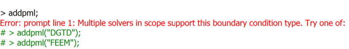
|
Example 2
The following script commands will add a PML boundary condition to the 'DGTD' solver, name it, and set the values for sigma and alpha.
adddgtdsolver;
addpml({"name":"simple_pml", "sigma":5});
| NOTE: The PML boundary condition automatically gets applied to the shell regions in the corresponding simulation region.
|
addabsorbing - Script command
Adds an absorbing boundary condition to the 'DGTD' solver. A DGTD solver region must be present in the objects tree for this command to work.
| Syntax | Description |
|---|---|
| addabsorbing; | Adds a PML boundary condition to the 'DGTD' solver. This function does not return any data. |
Example 1
The following script commands will add an absorbing boundary condition to the 'DGTD' solver already present in the objects tree and print all available properties of the boundary condition.
addabsorbing;
?set;
Example 2
The following script commands will add an absorbing boundary condition to the 'DGTD' solver, name it, and assign it to the -z and +z boundaries of the simulation region.
addabsorbing;
set("name","absorbing_z");
set("surface type","simulation region");
set("z min",1);
set("z max",1);
addperiodic - Script command
Adds a periodic (or Bloch) boundary condition to the 'DGTD' solver in Finite Element IDE. A DGTD solver region must be present in the objects tree for this command to work.
| Syntax | Description |
|---|---|
| addperiodic; | Adds a periodic boundary condition to the 'DGTD' solver. This function does not return any data. |
Example 1
The following script commands will add a periodic boundary condition to the 'DGTD' solver already present in the objects tree and print all available properties of the boundary condition.
addperiodic;
?set;
Example 2
The following script commands will add a periodic boundary condition in the x direction of the 'DGTD' solver.
addperiodic;
set("x periodic",1);
addpec - Script command
Adds a PEC (perfect electrical conductor) boundary condition to the DGTD or FEEM solver in Finite Element IDE. A DGTD or FEEM solver region must be present in the objects tree for this command to work. If both solvers are present then the intended solver's name must be provided as an argument to the script command.
| Syntax | Description |
|---|---|
| addpec; | Adds a PEC boundary condition to the DGTD or FEEM solver (whichever is present in the objects tree). This function does not return any data. |
| addpec("solver_name"); | Adds a PEC boundary condition to the desired solver defined by the argument "solver_name". The options are "DGTD" and "FEEM". This function does not return any data. |
Example 1
The following script commands will add a PEC boundary condition to the solver already present in the objects tree and print all available properties of the boundary condition.
addpec;
?set;
Example 2
The following script commands will add a PEC boundary condition to the DGTD solver, name it, and assign it to the -x and +x boundaries of the simulation region.
addpec("DGTD");
set("name","PEC_x");
set("surface type","simulation region");
set("x min",1);
set("x max",1);
addpmc - Script command
Adds a PMC (perfect electrical conductor) boundary condition to the DGTD or FEEM solver in Finite Element IDE. A DGTD or FEEM solver region must be present in the objects tree for this command to work. If both solvers are present then the intended solver's name must be provided as an argument to the script command.
| Syntax | Description |
|---|---|
| addpmc; | Adds a PMC boundary condition to the DGTD or FEEM solver (whichever is present in the objects tree). This function does not return any data. |
| addpmc("solver_name"); | Adds a PMC boundary condition to the desired solver defined by the argument "solver_name". The options are "DGTD" and "FEEM". This function does not return any data. |
Example 1
The following script commands will add a PMC boundary condition to the solver already present in the objects tree and print all available properties of the boundary condition.
addpmc;
?set;
Example 2
The following script commands will add a PMC boundary condition to the DGTD solver, name it, and assign it to the -y and +y boundaries of the simulation region.
addpmc("DGTD");
set("name","PMC_y");
set("surface type","simulation region");
set("y min",1);
set("y max",1);
addemeport - Script command
Adds a port to an EME solver region/object. The EME solver object must be set as the active solver for this command to work.
| Syntax | Description |
|---|---|
| addemeport; | Add a port to the active EME solver region. This function does not return any data. |
Example
The following script command will add a port to the EME solver region. The setactivesolver command is first used to set the EME solver region as the active solver.
setactivesolver("EME");
addemeport;
adddope - Script command
Adds a constant doping object to the simulation environment. This command requires a CHARGE solver region to be present in the objects tree.
| Syntax | Description |
|---|---|
| adddope; | Add a constant doping region. This function does not return any data. |
Example
The following script command will add a p-type constant doping object and set its dimension and concentration.
adddope;
set("name","pwell");
set("dopant type","p");
set("concentration",1e25);  # SI unit (/m3)
set("x",0);
set("x span",2e-6);
set("y",0);
set("y span",1e-6);
set("z",5e-6);
set("z span",1e-6);
adddopinglayer - Script command
Adds a doping layer to the layer builder object. The command only works if there is a layer builder object and is selected.
| Syntax | Description |
|---|---|
| adddopinglayer; | Adds a doping layer to the selected layer builder object. The name of the layer is set to "default name". This function does not return any data. |
| adddopinglayer("name"); | Adds a doping layer named "name" |
Example
The following script commands will create a layer builder object and add two doping layers to it.
addlayerbuilder;
#Doping Layer 1 = P doped layer
adddopinglayer("P");
setlayer("P", "dopant", "p");
setlayer("P", "concentration", 1e17);
#Doping Layer 2 = N++ doped layer
adddopinglayer("N++");
setlayer("N++", "dopant", "n");
setlayer("N++", "concentration", 1e19);
adddiffusion - Script command
Adds a diffusion doping region to the simulation environment. This command requires a CHARGE solver region to be present in the objects tree.
| Syntax | Description |
|---|---|
| adddiffusion; | Add a diffusion doping region in the simulation environment. This function does not return any data. |
Example
The following script command will add a n-type diffusion doping object and set its properties. The face where the dopants are introduced is defined by the "source face" property and the peak doping is defined by the "concentration" property. The "junction width" property defines the distance over which the doping drops from the (peak) concentration to the low "ref concentration" at the other faces of the doping object.
adddiffusion;
set("name","nwell");
# set dimensionset("x",0);
set("x span",2e-6);
set("y",0);
set("y span",1e-6);
set("z",5e-6);
set("z span",1e-6);
# set doping profile
set("dopant type","n");
set("source face",6);  # upper z
set("junction width",0.2e-6);
set("concentration",1e25);  # SI unit (/m3)
The figure below shows the resulting doping profile.
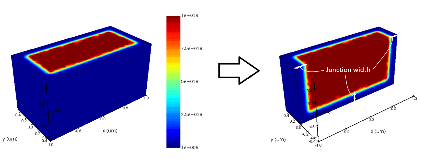
More information about the doping object itself, including the diffusion parameters can be found in this article.
addimport - Script command
Adds an import primitive to the simulation environment. The import primitive can be used to create a 3D geometry by importing a surface, an image, or binary data. It can also be used to create an n,k material.
| Syntax | Description |
|---|---|
| addimport; | Adds an import primitive to the simulation environment. This function does not return any data. |
Example
The following script commands will generate a surface data and then use the data to create a layer of glass whose top surface is defined by the generated data.
# generate a surface
nx = 50;
ny = 40;
x = linspace(-6,6,nx);
y = linspace(-5,5,ny);
X = meshgridx(x,y);
Y = meshgridy(x,y);
Z = exp(-(X^2+Y^2)/4^2) * sin(pi*Y/2);
# Remember that all units are SI. We defined the surface in microns
# so all lengths must be multiplied by 1e-6
x = x*1e-6; # switch to SI units
y = y*1e-6; # switch to SI units
Z = Z*1e-6; # switch to SI units
# create substrate layer with an import object
addimport;
set("material","SiO2 (Glass) - Palik");
# upper surface and reference height
importsurface2(Z,x,y,1);
set("upper ref height",0e-6);
addbulkgen - Script command
Adds a bulk (optical) generation region to the simulation environment. The bulk generation (source) object can be used to create an analytic solar generation profile. This command requires a CHARGE solver region to be present in the objects tree.
| Syntax | Description |
|---|---|
| addbulkgen; | Add a bulk (optical) generation region. This function does not return any data. |
Example
The following script commands will add a bulk generation (source) object to the CHARGE solver region. The object is set up to calculate the solar generation rate in silicon considering the AM1.5G solar spectrum.
addbulkgen;
set("name","solar");# set dimension
set("x",0);
set("x span",2e-6);
set("y",0);
set("y span",1e-6);
set("z",5e-6);
set("z span",1e-6);
# set parameters for analytic profile
set("illumination face",6);  #  upper z
set("spectrum",0);  # AM1.5G
set("material",0);  # silicon
set("interface reflection",1);  # air interface
adddeltachargesource - Script command
Adds a delta optical generation source to the simulation environment. This command requires a CHARGE solver region to be present in the objects tree.
| Syntax | Description |
|---|---|
| adddeltachargesource; | Add a delta optical generation source to the simulation environment. This function does not return any data. |
Example
The following script commands will add a delta optical generation source, set its location, and set the generation rate by defining a net electron-hole-pair current (/sec).
adddeltachargesource;
set("name","delta");
set("x",0);
set("y",0);
set("z",5e-6);
set("source type",2);  #  ehp current
set("ehp current",1e12);  # net ehp current I_ehp = e*1e12 Amp
addimportdope - Script command
Adds a doping region to the simulation environment that can be used to load a custom doping profile. The custom doping profile can be created analytically using script or it can be imported from other sources such as process simulation. This command requires a CHARGE solver region to be present in the objects tree.
| Syntax | Description |
|---|---|
| addimportdope; | Add an import doping region to the simulation environment. This function does not return any data. |
Once the import doping object is created, the doping data can be imported from a matlab (.mat) file using the GUI or by assigning a dataset to the object using the importdataset script command. The dataset can be a rectilinear or an unstructured dataset. Doping data can be imported into the solver workspace from other tools (e.g. process simulation) using the Dataset builder .
Example
The following script command will add an import doping object to the CHARGE solver region and will load an analytic 3D doping data into it.
addimportdope;
set("name","pepi");
set("x",0);
set("y",0);
set("z",0);
# create coordinate vectors and 3D matrix for doping profile
x = linspace(0,1e-6,11);
y = linspace(-1e-6,1e-6,2);
z = linspace(0,2e-6,101);
N = matrix(11,2,101) + 1e21;  # assume uniform doping concentration of 1e15 /cm3 (1e21 /m3)
# create dataset
doping = rectilineardataset("dope",x,y,z);
doping.addparameter("a",1);  # add a dummy parameter
doping.addattribute("N",N);
# load data into doping object
select("CHARGE::pepi");
importdataset(doping);
addimportgen - Script command
Adds an (optical) generation region to the simulation environment where the generation profile has been imported into Finite Element IDE. This command requires a CHARGE solver region to be present in the objects tree.
| Syntax | Description |
|---|---|
| addimportgen; | Add an import generation object to the simulation environment. This function does not return any data. |
Once the import generation object is created, the optical generation data can be imported from a matlab (.mat) file using the GUI or by assigning a dataset to the object using the importdataset script command. The .mat file must contain a 3D matrix G containing the generation data on a rectilinear grid and the three coordinate vectors x, y, z. The dataset can be either a rectilinear or an unstructured dataset.
Example
The following script command will add an import generation object to the CHARGE solver region and will load an analytic 3D optical generation data into it.
addimportgen;
set("name","gen_opt");
set("x",0);
set("y",0);
set("z",0);
# create coordinate vectors and 3D matrix for doping profile
x = linspace(0,1e-6,11);
y = linspace(-1e-6,1e-6,2);
z = linspace(0,2e-6,101);
G = matrix(11,2,101) + 1e27;  # assume uniform generation rate of 1e21 /cm3 (1e27 /m3)
# create dataset
gen = rectilineardataset("gen",x,y,z);
gen.addparameter("a",1);  # add a dummy parameter
gen.addattribute("G",G);
# load data into doping object
select("CHARGE::gen_opt");
importdataset(gen);
adduniformheat - Script command
Adds a constant heat source to the HEAT solver region. The input is defined as the net heat input to the volume in units of Watt. The uniform heat source can either be 2D or 3D. The heat input per unit volume (W/m 3 ) is calculated by dividing the net input power by the volume of the (3D) source. In the case of a 2D source the volume of the source is defined by setting the length in the third dimension equal to either the "equivalent length" of the source or the "norm length" of the HEAT solver.
| Syntax | Description |
|---|---|
| adduniformheat; | Adds a constant heat source to the simulation environment. This function does not return any data. |
Example
The following script adds a 3D uniform heat source to the HEAT solver, sets its dimension, and assigns a net input power.
adduniformheat;  # the dafult format of a newly created heat source is 3D

set("x",0);
set("x span",2e-6);
set("y",0);
set("y span",5e-6);
set("z",0);
set("z span",10e-6);
set("total power",1e-4);  #  Pin = 0.1 mW
The following script adds a 2D y-normal uniform heat source to the HEAT solver, sets its dimension, forces the length in the third dimension to be equal to the "norm length" of the HEAT solver, and assigns a net input power.
adduniformheat;

set("source type",2);  # 2D y-normal
set("use solver norm length",1);
set("x",0);
set("x span",2e-6);
set("y",0);
set("z",0);
set("z span",10e-6);
set("total power",1e-4);  #  Pin = 0.1 mW
addimportheat - Script command
Adds a heat source to the Finite Element IDE simulation environment where the profile of the heat source can be imported from an external source. For the CHARGE solver, the import heat source only gets applied if the "temperature dependence" is set to "coupled."
| Syntax | Description |
|---|---|
| addimportheat; | Adds an import primitive to define a heat source. This format of the command is only application when only one solver is present/active in the model tree. This function does not return any data. If multiple solvers are present then use the second format. |
| addimportheat("solver_name"); | This format of the command will add an import heat source to the solver defined by the argument. The "solver name" will be either “CHARGE” or “HEAT.” |
Once the import heat source is created, the data can be imported from a matlab (.mat) file using the GUI or by assigning a dataset to the object using the importdataset script command. The dataset can be in rectilinear or unstructured (finite-element) format.
Example
The following script command will add an import heat source to the HEAT solver region and will load an analytic 3D heat data into it.
addimportheat("HEAT");
set("name","Pin");
# create coordinate vectors and 3D matrix for heat input
x = linspace(0,1e-6,11);
y = linspace(-1e-6,1e-6,2);
z = linspace(0,2e-6,101);
Q = matrix(11,2,101) + 1e15;  # assume the heat input is 1e15 W/m^3 everywhere
# create dataset
heat = rectilineardataset("Pin",x,y,z);
heat.addparameter("a",1);  # add a dummy parameter
heat.addattribute("Q",Q);
# load data into source
select("HEAT::Pin");
importdataset(heat);
addimporttemperature - Script command
Adds an import temperature source to the CHARGE solver (only applicable to non-isothermal transport). The import temperature object can be used to import a temperature map for non-isothermal simulation. A CHARGE solver region must be present in the objects tree for this command to work.
| Syntax | Description |
|---|---|
| addimporttemperature; | Adds an import temperature source to the CHARGE solver. The source only gets applied if the "temperature dependence" is set to "non-isothermal." This function does not return any data. |
Once the import temperature source is created, the data can be imported from a matlab (.mat) file using the GUI or by assigning a dataset to the object using the importdataset script command. The dataset can either be in rectilinear or unstructured (finite-element) format.
Example
The following script command will add an import temperature source and will load an analytic 3D temperature data into it.
addimporttemperature;
set("name","Tmap");
# create coordinate vectors and 3D matrix for temperature map
x = linspace(0,1e-6,11);
y = linspace(-1e-6,1e-6,2);
z = linspace(0,2e-6,101);
T = matrix(11,2,101) + 400;  # assume the temperature is 400 K everywhere
# create dataset
temperature = rectilineardataset("temp",x,y,z);
temperature.addparameter("a",1);  # add a dummy parameter
temperature.addattribute("T",T);
# load data into source
select("CHARGE::Tmap");
importdataset(temperature);
addimportnk - Script command
Adds a nk import object to the FEEM simulation environment where the profile of the material with a spatially varying index can be imported from an external Matlab file.
| Syntax | Description |
|---|---|
| addimportnk; | Adds an import primitive to define material with a spatially varying index profile in the FEEM solver. This function does not return any data. |
Once the nk import object is created, the data can be imported from a matlab (.mat) file using the GUI or by assigning a dataset to the object using the importdataset script command. The dataset can be in rectilinear or unstructured (finite-element) format.
Example
The following script command will add an import (n,k) object to the FEEM solver region and will load an analytic 3D heat data into it.
addfeemsolver;
addimportnk;
# create coordinate vectors and 3D matrix for nk input
x = linspace(0,1e-6,11);
y = linspace(-1e-6,1e-6,2);
z = linspace(0,2e-6,101);
nk = matrix(11,2,101)+3.45; # assume the index input is 3.45 everywhere
for (i=1:length(x)){
# assume that index varies along x-axis
nk(i,:,:)=x(i)*1e5;}
# add waveguide
addrect;
setname('WG');
set('x min',-1e-6);
set('x max',1e-6);
set('y span',2e-6);
set('y',0);
set('z span',2e-6);
set('z',1e-6);
# create dataset
nkmaterial = rectilineardataset("nk import",x,y,z);
nkmaterial.addparameter("lambda",1.55e-6); # (Required) add any parameter
nkmaterial.addattribute("nk",nk);
# load data into nk import
select("FEEM::nk import");
importdataset(nkmaterial);
set("volume type","solid");
set("volume solid","WG");
set("selected attribute","nk");


 565
565

 被折叠的 条评论
为什么被折叠?
被折叠的 条评论
为什么被折叠?
 到【灌水乐园】发言


