FDTD product reference manual-Optimizations and sweeps

weixin_43044416

已于 2023-09-05 10:09:45 修改

阅读量1.2k

点赞数 1

文章标签：学习

于 2023-08-29 16:23:33 首次发布

本文链接：https://blog.csdn.net/weixin_43044416/article/details/132558371

版权

Learn how to run parameter sweep, optimization, yield analysis, and s-parameter analysis tasks.

Parameter sweep utility

FDTD RCWA MODE DGTD CHARGE HEAT FEEM INTERCONNECT

This page describes how to run a parameter sweep using the built in sweep utility. Parameter sweeps are useful for finding the optimum value of a parameter, and for studying the sensitivity of the design performance to certain parameters or running a series of simulations with a set of varying parameters. We will demonstrate how to use the parameter sweep feature in a simple example: finding the optimum thickness of an anti-reflection (AR) layer on silicon. The optimum thickness is the thickness that gives the minimum reflection at the wavelength of operation, which in this example is 500 nm.

Parameter sweep properties

NAME: Parameter sweep name.

Parameters

TYPE- RANGES: Specify sweep points with start / stop values. All values will be linearly spaced.
TYPE - VALUES: Specify each sweep point manually. Allows non-linearly spaced sweep values.
NUMBER OF POINTS: Number of points in the parameter sweep.
NAME: A user specified name for the parameter. Will appear in results dataset.
PARAMETER: Property to sweep.
TYPE: Used to specify the type of units for the selected property (eg. length, time).
START/STOP: The start/stop value of the sweep, when using the RANGES option.
VALUE_1,2,3,...: Specific sweep values, when using the VALUES option.
ADD: Add another line to the parameters table.
REMOVE: Remove a line from the parameters table.

Results

NAME: A user specified name for the result. Will appear in the results dataset.
RESULT: Result to collect.
OPERATION: Optionally, apply a simple mathematical operation to the results. Supported operations are Sum, Mean, Integrate.

Advanced

RESAVE FILES AFTER ANALYSIS: Optionally, resave the project files after the analysis scripts have been run. This can be helpful when the analysis scripts are slow to run.

Creating a parameter sweep project

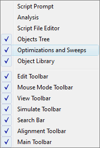
1. Make sure you can see the Optimization and Sweeps window. This can be done by going to the menu View->Windows->Optimization and Sweeps, or by right clicking on the upper menu bar and making sure that Optimization and sweeps is selected.

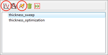
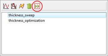
2. Click the Add Sweep button to create a new parameter sweep task. Click the edit button to open the Edit sweep dialog window.

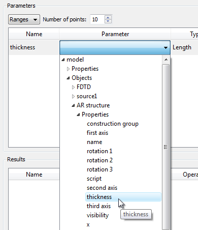
3. Editing parameters

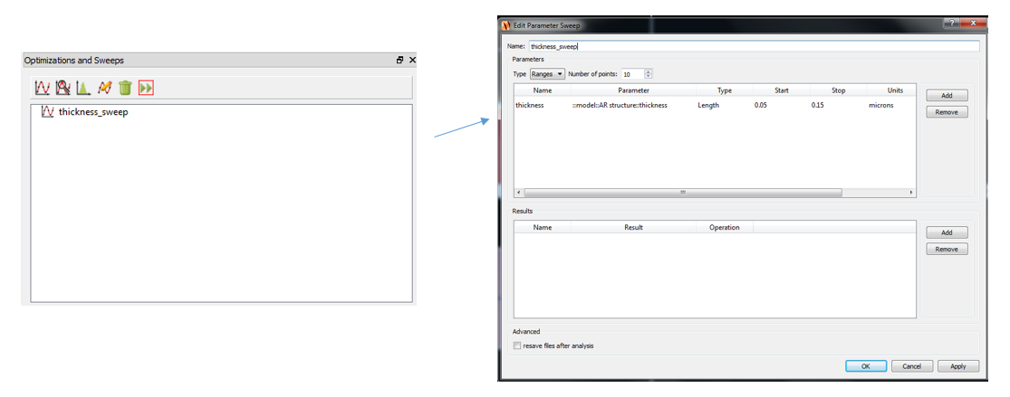
Once the sweep object is open, add a parameter and browse the parameter pulldown menu. Select the "thickness" property of the AR structure.

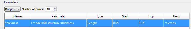
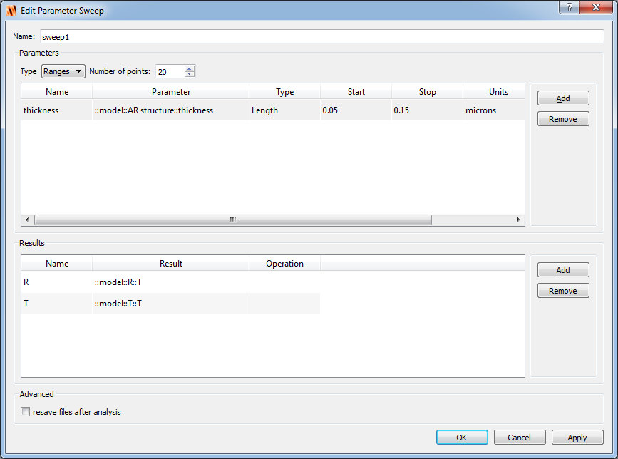
4. Next, choose the Type to be length and set the Start and Stop values to 10nm and 150nm respectively. The final result should look like the screenshot here.

NOTE: Multiple parameter sweeps and Nested Sweeps

If two or more parameters are specified, they must have the same dimensions (i.e., number of points). Each sweep step will update all parameters values one column at a time (this is not the same as nested parameter sweeps). For information on how to set up nested parameter sweeps, please see Nested Sweeps.

5. Recording results

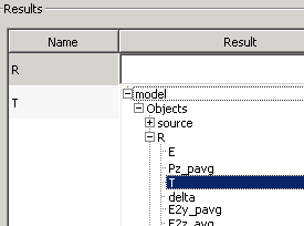
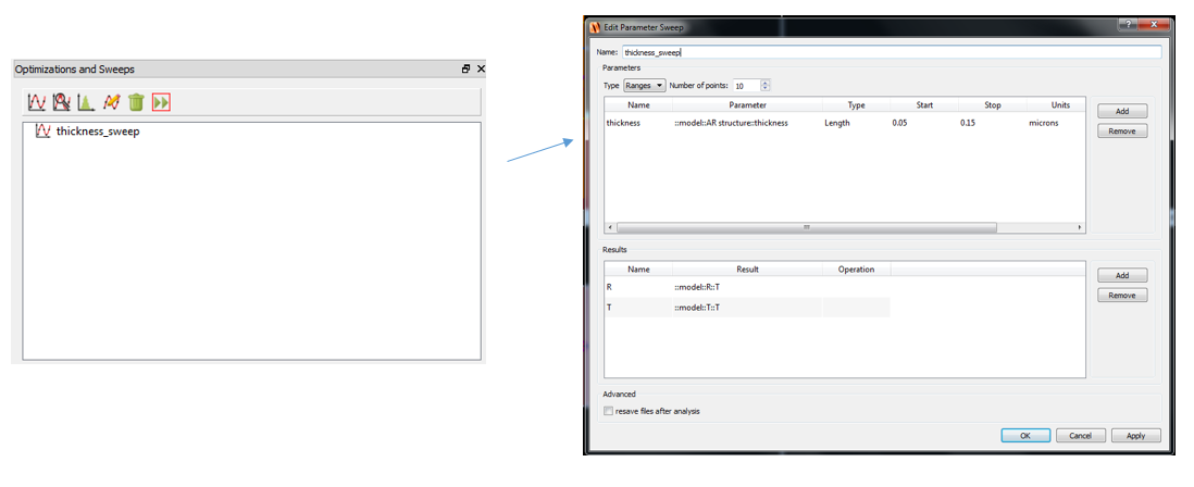
Add results to record, the recorded results will be available when the sweep is done. Select the power transmission 'T' from the Reflection and Transmission monitors, as shown here.

6. Under the Operation column, please leave the choice blank. The final Parameter Sweep window should look like this figure. Click OK to accept all settings, and go back to the main Optimization and Sweeps window.

NOTE: File not found!

Ensure that there is no period in the parameter sweep name. Otherwise it may result in "file not found" error while running the sweep.

Running the parameter sweep

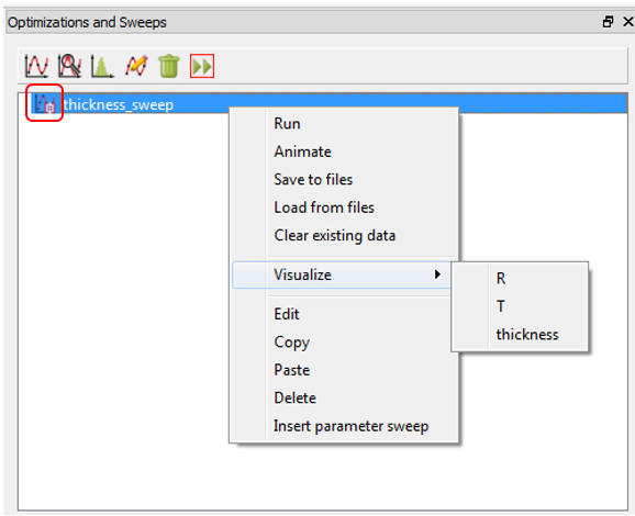
To run the parameter sweeps, select the parameter sweep and click the run button. To distribute the sweep between several local computers, you must configure the computation Resources before running the optimization. Without additional configuration, all simulations will run on the local computer.

Viewing the results

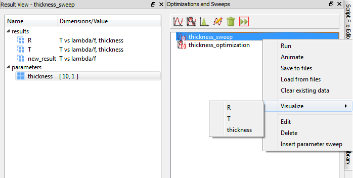
The parameter sweep data is saved in a similar way to monitor data. One can right-click on the results in the Result View or the parameter sweep project to select any of the sweep results to be displayed in the Visualizer.

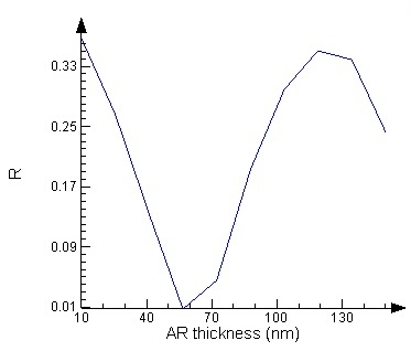
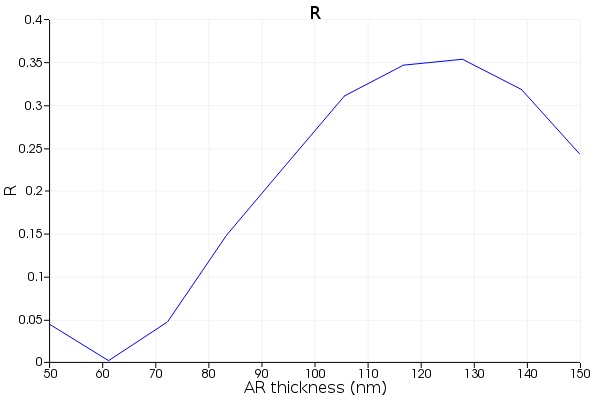
Parameter sweep results can also be obtained in the script environment with the command getsweepresult, which is similar to the command getresult. The name of each data member is the Name column that you specified when adding the parameters and results, in this case "T", "R" and "thickness". For example, the following 2 lines of script will plot the result R vs thickness.

R = getsweepresult("thickness_sweep","R");
plot(R.thickness*1e9, R.T, "AR thickness (nm)","R");

We can see that the best thickness is approximately 60 nm. To find the precise value, we could repeat the parameter sweep with more points, or reduce the range of the thicknesses we consider. Alternatively, we could consider using an Optimization project (Optimize a design) to find the thickness that gives the smallest reflection.

Creating parameter sweeps using a script

FDTD MODE DGTD CHARGE HEAT FEEM INTERCONNECT

This page describes how to generate and run a sweep using script commands. The script commands used in this example could also be applied to optimization and yield analysis.

To generate and run the sweep using script commands, user can open the sweep_AR_coating_example_script.fsp file and follow the three steps listed below; or, open and run the script file sweep_AR_coating_example_script.lsf.

Creating the parameter sweep project

The following commands are used to generate and superficially define a new sweep named "thickness_sweep_script".

# add a new sweep and set basic properties
addsweep;
setsweep("sweep", "name", "thickness_sweep_script");
setsweep("thickness_sweep_script", "type", "Ranges");
setsweep("thickness_sweep_script", "number of points", 10);

When the sweep is superficially generated, the parameters can then be defined and added to it. The following commands define the name, type, range and the path of the parameter "thickness".

# define the parameter thickness
para = struct;
para.Name = "thickness";
para.Parameter = "::model::AR structure::thickness";
para.Type = "Length";
para.Start = 0.05e-6;
para.Stop = 0.15e-6;
para.Units = "microns";

This command adds the parameter "thickness" to the sweep "thickness_sweep_script". When the parameter is successfully added, the sweep will appear in the "Optimizations and Sweeps" tab as shown below.

# add the parameter thickness to the sweep
addsweepparameter("thickness_sweep_script", para);

The next step is to add the results that we want to measure into the sweep. The commands listed below define and add the results "R" and "T" to the sweep as shown in the sweep editing window below. After this step, the sweep is well defined and ready to run.

# define results
result_1 = struct;
result_1.Name = "R";
result_1.Result = "::model::R::T";

result_2 = struct;
result_2.Name = "T";
result_2.Result = "::model::T::T";

# add the results R & T to the sweep
addsweepresult("thickness_sweep_script", result_1);
addsweepresult("thickness_sweep_script", result_2);

Running the parameter sweep

A well defined sweep can also be run by using script commands. The following command runs the sweep "thickness_sweep" and loads the results to it. After running, the results will be loaded back to the sweep and the sweep will be indicated by the red logo as shown below.

# run the sweep
runsweep("thickness_sweep_script");

Viewing the results

The sweep results could also be visualized by using script commands. The commands below stores the sweep results "R" and "T" to two same named datasets "R" and "T" and plots them.

# save & view the results
R = getsweepresult("thickness_sweep_script", "R");
T = getsweepresult("thickness_sweep_script", "T");

plot(R.thickness*1e9, R.T, "AR thickness (nm)","R");
# T is in the opposite direction of R
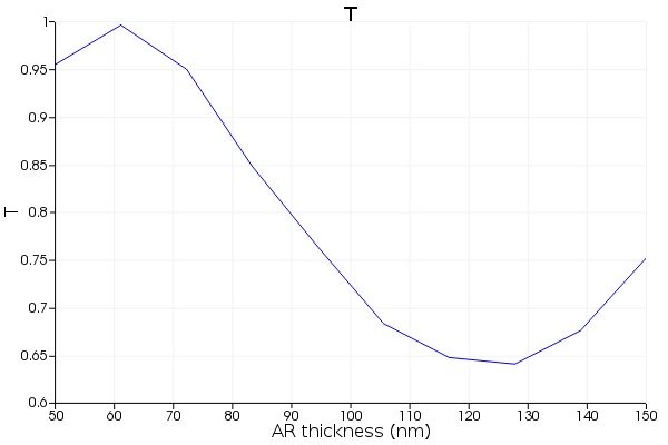
plot(T.thickness*1e9, abs(T.T), "AR thickness (nm)","T");

The following figures are the plots of the results R and T v.s. thickness, which show same results as in the section Parameter sweeps.

Creating nested parameter sweeps

FDTD MODE DGTD CHARGE HEAT FEEM INTERCONNECT

This section describes how to create and run a nested parameter sweep. We will demonstrate how to do this by finding the incident angle that results in minimum reflection from a 50 nm silver film on glass for 3 different wavelengths (for a more detailed description of this example, see Surface Plasmon Resonance 2D).

Creating the nested parameter sweep project

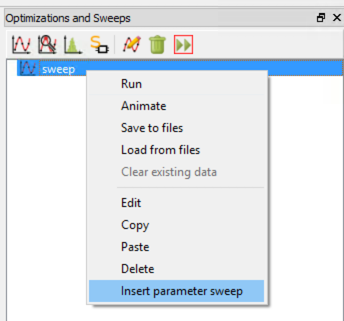
In the Optimization and Sweeps window, click the Add Sweep button to create a new parameter sweep task (see Parameter sweeps). Once the sweep is added, right click on the new sweep project and select Insert Parameter Sweep.

A nested parameter sweep will be created as a result. Open the edit window for the inner sweep object, change the name to "theta", add a parameter "source_angle" and browse the parameter pulldown menu to select the "angle" property of the source. Set the Start/Stop values to sweep from 40 to 60 degrees, and the Number of points 20. Finally, add a result "R" from the reflection analysis group (see Creating parameter sweep for step-by-step details). The edit window should look like the screenshot below.

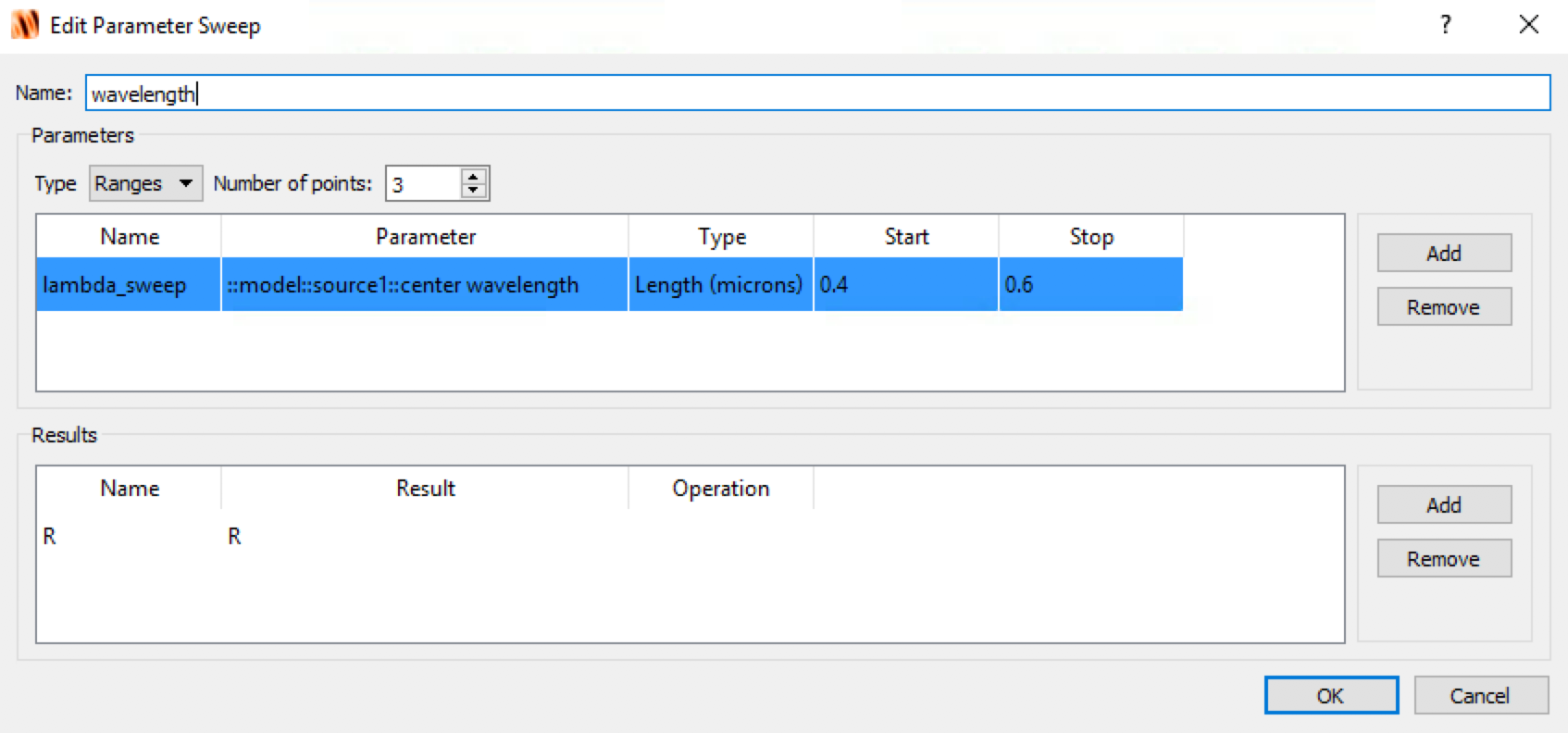
In the edit window for the outer sweep, change the name to "wavelength", add a parameter "lambda" and browse the parameter pull down menu to select the "wavelength" property of the source. Set the Start/Stop values to sweep from 0.4 to 0.6 microns in 3 points. Add a result "R" and select R from the Result pull down menu, which contains all the results in the inner sweep that are already defined.

Running the nested parameter sweep

The nested parameter sweep can be run in the same manner as a single parameter sweep, as described in Parameter sweeps.

Viewing the results

Just like single parameter sweeps, the data from a nested parameter sweep can also be retrieved using getsweepresults. The following commands can be used to plot the data. It is also possible to plot this data with the visualizer.

reflection = getsweepresult("wavelength", "R"); 
R =     -reflection.T;
lambda = reflection.lambda_sweep*1e9;

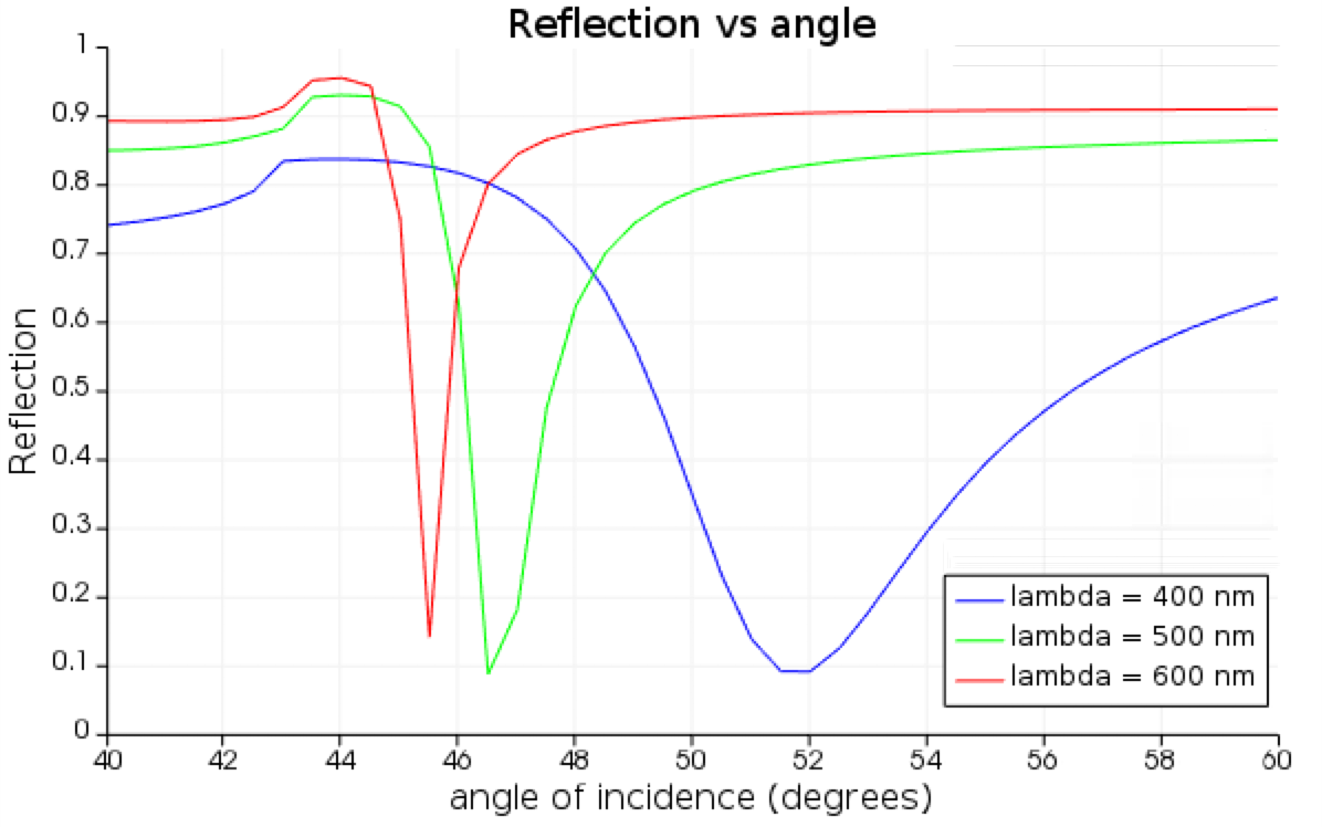
plot(reflection.source_angle, pinch(R,2,1), pinch(R,2,2), pinch(R,2,3),
     "angle of incidence (degrees)","Reflection","Reflection vs angle");
legend('lambda = ' + num2str(lambda(1)),
       'lambda = ' + num2str(lambda(2)),
       'lambda = ' + num2str(lambda(3)));

We can see that shorter wavelengths correspond to larger incident angles where minimum reflection is obtained.

Note: Optimizations with nested sweeps

This example file also contains an optimization task with a nested sweep. The optimization task is setup to find the optimal thickness of silver to minimize the reflected power for illumination by 500 nm light at angles between 45 and 50 degrees. The nested sweep is used to calculate the average reflection for angles between 45 and 50 degrees for each design (ie. thickness) in the optimization.

Running parameter sweeps without the CAD

FDTD MODE DGTD CHARGE HEAT FEEM INTERCONNECT

This section describes an alternative way to run parameter sweeps on a separate network (i.e. an external cluster). If your full license is installed on one network (i.e. your office) and your extra engine licenses are installed on an external cluster, then the Job Manager feature of FDTD can't be used. Instead, you will use the full license on your local computer to generate a set of simulation files. These files are then transferred to the cluster. Very often, these jobs will be submitted to the clusters job scheduler. See the Running simulations section for more information on running simulations from the command line (i.e without using the Lumerical Job Manager). When the simulations are finished, the files are transferred back to the local desktop computer. You can then reload the data files and extract the requested information.

Adjust model parameters and save a set of fsp files (a fsp file for each parameter value).
Run all the simulations
Load the simulation files and extract the required information

Advantages: The individual simulations can be sent to an external cluster or other workstations

Disadvantages: It is not quite as simple to run all the simulations

Step 1: Adjust model parameters and save a new fsp file for each parameter value

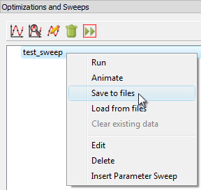
After setting up a parameter sweep as described at Parameter sweeps, rather than running the parameter sweep directly, simply choose Save to files, as shown below.

This will create a directory called with the same name as the original fsp file, in this case, usr_optimization_example. Inside this directory you will find 10 fsp file, called "test_sweep_1.fsp" to "test_sweep_10.fsp". Each file corresponds to a particular value of the parameters and there are 10 files because we chose 10 different values for our sweep parameter.

Step 2: Run the simulations

The simulations can be run on a cluster or extra workstations, without requiring a graphical user interface license. A shell or job scheduler is the most convenient way to run these simulations. For further details, see Resource configuration in the Installation category. In particular, Running from the command line using MPI for your operating system, or Job scheduler submission scripts (SGE, Slurm, Torque).

Step 3: Load the results

Once all the simulations have been completed, you can load all the results by choosing Load from files, as shown below.

This will reload all the results from the fsp files, as if they had been run on the local machine by pressing the Run button. You can then proceed with the analysis of the results as shown in Parameter sweeps.

Note: Re-running the parameter sweep

Once the sweep is run, a new set of fsp files are saved to a folder. If the sweep is run again, then a set of fsp files will be saved to overwrite t