


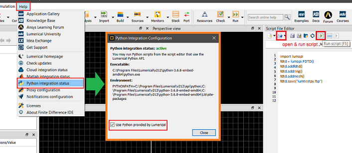
Use Python to analyze data, automate complex workflows\optimizations, and produce publication-quality plots. Lumerical's inverse design optimization makes extensive use of the Python API. The API can be used for developing scripts or programs that treat Lumerical solvers as clients, or in high-performance computing settings where performance and license utilization are imperative.
Python v3 is included with Lumerical's software, which avoids the need for any complex setup or configuration.
Requirements
- Lumerical product version 2019a R3 or later
- Gnome or Mate desktop environment for supported Linux systems when running from the Lumerical CAD/GUI.
- A graphical interface/connection to the machine running the API
- A Lumerical GUI license.
Note: The Python API requires interfacing with the Lumerical GUI and will utilize a GUI license.
Getting Started
Session management - Python API

This article demonstrates the feasibility of integrating Lumerical tools with Python to develop complex automated workflows and perform advanced data processing/plotting. Interoperability is made possible using the Python API, a python library known as lumapi. Hereafter these terms will be used interchangeably. Users will develop methods of managing a Lumerical session, and learn techniques of initializing and editing Lumerical simulation objects from Python script.
It should be possible to store the files in any working directory; however, it is recommended to put the Lumerical and Python files in the same folder. Basic commands for appending the environment path are given in Setting the Python Before Importing, but sophisticated manipulation of the directories is beyond the scope of this article. To modify the Lumerical working directory find instructions here.
A connection to the lumapi.py file is the key to enabling the Lumerical-Python API interface. This is accomplished by importing the lumapi module, and initializing a session. When initializing a session this will consume a GUI license. Accessing simulation objects is discussed below. Using script commands, and passing data are discussed in the articles Script commands as methods - Python API, and Passing Data - Python API.
Importing Modules
Python Path is Configured
For convenience, a basic Python 3 distro is shipped with Lumerical's solvers allowing users to get started immediately; by running any of our examples from the CAD script editor where lumapi can be loaded like any module.
import lumapi
Many users would like to integrate lumapi into their own Python environment. This is as simple as importing the lumapi module; however, by default python will not know where to find it. This can be addressed by modifying the search path. Please refer to the Python foundations guide on installing modules. Essentially we allow Python to find the lumapi module, by including its parent directory in the list that import class will search. Usually, a one-time update, see explicit path import for the OS specific directories. If you are not ready or to update the Python path then either of the following methods should work
Adding the Python Before Importing
To temporarily add the lumapi directory to your path, you can use the sys.path.append() method. This is the case if you have not yet added lumapi to your search path, and it is also useful when adding directories of other helpful lsf, fsp, py files. The following code adds the lumapi folder and current file directory.
Windows:
import sys, os
#default path for current release
sys.path.append("C:\\Program Files\\Lumerical\\v232\\api\\python\\")
sys.path.append(os.path.dirname(__file__)) #Current directory
Linux:
import sys, os
#default path for current release
sys.path.append("/opt/lumerical/v232/api/python/lumapi.py")
sys.path.append(os.path.dirname(__file__)) #Current directory
Explicit Import
If you need to specify the path to your lumapi distribution then the importlib.util() is the best method for pointing to the lumapi module. This may be the case if you are working on a different branch, or comparing lumapi versions.
Windows:
import importlib.util
#default path for current release
spec_win = importlib.util.spec_from_file_location('lumapi', 'C:\\Program Files\\Lumerical\\v232\\api\\python\\lumapi.py')
#Functions that perform the actual loading
lumapi = importlib.util.module_from_spec(spec_win) #windows
spec_win.loader.exec_module(lumapi)
Linux:
import importlib.util
#default path for current release
spec_lin = importlib.util.spec_from_file_location('lumapi', "/opt/lumerical/v232/api/python/lumapi.py")
#Functions that perform the actual loading
lumapi = importlib.util.module_from_spec(spec_lin)
spec_lin.loader.exec_module(lumapi)
See also: How to run Lumerical API (Python) scripts in Linux – Ansys Optics
Starting a session
This is as simple as calling the relevant constructor for the Lumerical product and storing it in an object.
fdtd = lumapi.FDTD()
Since the 2023 R1.2 release, the Python API can be used remotely on a Linux machine running the interop server (see Interop Server - Remote API to configure and run the interop server). To use the remote API, an additional parameter is required when starting a session, to specify the IP address and port to use to connect to the interop server. This port has to be the starting port defined for the interop server.
This parameter is an dictionary with 2 fields, "hostname" and port.
remoteArgs = { "hostname": "192.168.215.129",
               "port": 8989 }
fdtd = lumapi.FDTD(hide=True, remoteArgs=remoteArgs)
You can create multiple sessions of the same product and different products at once, as long as they all have unique names.
mode1 = lumapi.MODE()
mode2 = lumapi.MODE()
device = lumapi.DEVICE()
Each of the product's constructor supports the following named optional parameters:
- hide (default to False): Shows or hides the lumerical GUI/CAD environment on startup
- filename (default empty): Launches a new application if it is empty, and will run the script if an lsf file is provided. If a project filename is provided; it will try and load the project if it can be found in the path. See the section setting the python path before importing to add folder or use the full path to load files from other directories.
# loads and runs script.lsf while hiding the application window
inc = lumapi.INTERCONNECT(filename="script.lsf", hide=True)
Import Methods
Besides defining methods/functions in Python, user can take advantage of the auto-syncing function feature in lumapi and import functions that are pre-defined in a Lumerical script file (.lsf file or format). Once the script has been excuted using the "eval" command, the methods can be called as pre-defined methods in lumapi.
Follow is an example of importing functions from a script file "testScript.lsf" and from a script format string.
fdtd = lumapi.FDTD()

# import function defined in script format string
fdtd .eval("function helloWorld() { return \"hello world\"; }\nfunction returnFloat() { return 1.; }\nfunction addTest(a, b){ return a*b; }")
print(fdtd .helloWorld())

# import function defined in the script file "testScript.lsf"
code = open('C:/XXX/testScript.lsf', 'r').read()
fdtd .eval(code)
The script can also be passed as a parameter in the constructor to define a method:
def testAddingMethodsFromConstructor(self):
app = self.appConstructor(script="any_product_script_workspace_functions_available_in_python_test.lsf")
expectedMethods = {'helloWorld'}
expectedResults = ['hello world from script file']
results = []
results.append(app.helloWorld())
self.assertEqual(results, expectedResults)
app.close()
Advanced session management
When the variables local to the function or context manager go out of scope, they will be deleted automatically, and a Lumerical session will automatically close when all variable references pointing to it are deleted.
Wrapping the session in a function
In Python you can use functions if you need to run numerous similar instances; for example, when sweeping over some optional parameters. For more information on how the important results are returned see Passing data - Python API.
def myFunction(someOptionalParameter):
    fdtd = lumapi.FDTD()
    ...
    return importantResult
Using the "with" context manager
We support Python "with" statement by giving well-defined entrance and exit behavior to Lumerical session objects in Python. If there was any error within the "with" code block, the session still closes successfully (unlike in a function). Also note that any error message you typically see in a Lumerical script environment would be displayed in the Python exception.
with lumapi.FDTD(hide=True) as fdtd:
    fdtd.addfdtd()
    fdtd.setnamed("bad name") ## you will see
LumApiError: "in setnamed, no items matching the name 'bad name' can be found."
    ...
## fdtd still successfully closes
Simulation Objects
Since the release of 2019a, Python API supports adding objects using a constructor and setting sim-objects from a constructor.
Adding simulation objects using a constructor
When adding an object, its constructor can be used to set the values of properties at creation.
fdtd.addfdtd(dimension="2D", x=0.0e-9, y=0.0e-9, x_span=3.0e-6, y_span=1.0e-6)
In Python, dict ordering is not guaranteed, so if there are properties that depend on other properties, an ordered dict is necessary. For example, in the below line of Python, 'override global monitor settings' must be true before 'frequency points' can be set.
props = OrderedDict([("name", "power"),("override global monitor settings", True),("x", 0.),("y", 0.4e-6),
                     ("monitor type", "linear x"),("frequency points", 10.0)])
fdtd.addpower(properties=props)
If you do not have properties with dependencies you can use regular Python dictionaries.
props = {"name": "power",
         "x" : "0.0",
         "y" : 0.4e-6",
          "monitor type" : "linear x"}
fdtd.addpower(properties=props)
Manipulating simulation-objects
When adding a new object to a Lumerical product session, a representative Python object is returned. This object can be used to make changes to the corresponding object in the Lumerical product.
rectangle = fdtd.addrect(x = 2e-6, y = 0.0, z = 0.0)
rectangle.x = -1e-6
rectangle.x_span = 10e-6
Dict-like access
The below line of python code shows an example of the dict-like access of parameters in an FDTD rectangle object.
rectangle = fdtd.addrect(x = 2e-6, y = 0.0, z = 0.0)
rectangle["x"] = -1e-6
rectangle["x span"] = 10e-6
Parent and children access
The tree of objects in a Lumerical product can be traversed using the parent or children of an object.
device.addstructuregroup(name="A")
device.addrect(name="in A")
device.addtogroup("A")
device.addstructuregroup(name="B")
device.addtogroup("A")
bRect = device.addrect(name="in B")
device.addtogroup("A::B")

# Go up two parents from the rectangle in "B" group
aGroup = bRect.getParent().getParent()

# Print the names of all members of "A" group
for child in aGroup.getChildren():
    print child["name"]
| Note: Python will automatically delete variables as they removed from scope, so most of the time you will not need to close a session manually. To do so explicitly, you can call the close session using. inc.close() #inc is the name of the active session |
Script commands as methods - Python API
FDTD MODE DGTD CHARGE HEAT FEEM INTERCONNECT Automation API
Almost all script commands in the Lumerical script language can be used as methods on your session object in Python. The lumapi methods and the Lumerical script commands share the same name and can be called directly on the session once it's been created. For example,
fdtd.addrect() # Note the added brackets since this is a method in Python.
For more information on Lumerical scripting language please see:
- Scripting Learning Track on Aansys Innovation Courses (AIC)
- Lumerical scripting language - Alphabetical list
- Lumerical scripting language - By category
Documentation Docstrings
For information on the lumapi methods from within the environment we support Python docstrings for Lumerical session objects. This is the simplest way to determine the available script commands, and syntax. This contains information that is similar to the Alphabetical List of Script Commands . You can view the docstring by using the Python built-in function "help" or most ways rich interactive Python shells display docstrings (e.g. IPython, Jupyter Notebook):
>>> help(f.addfdtd)
Help on method addfdtd in module lumapi:
addfdtd(self, *args) method of lumapi.FDTD instance
    Adds an FDTD solver region to the simulation environment.  The extent of
    the solver region determines the simulated volume/area in FDTD
    Solutions.
    +-----------------------------------+-----------------------------------+
    | Syntax                            | Description                       |
    +-----------------------------------+-----------------------------------+
    | o.addfdtd()                       | Adds an FDTD solver region to the |
    |                                   | simulation environment.           |
    |                                   |                                   |
    |                                   | This function does not return any |
    |                                   | data.                             |
    +-----------------------------------+-----------------------------------+
    See Also
    set(), run()
    https://kb.lumerical.com/en/ref_scripts_addfdtd.html
| Note: We still support previous version of the Python API, yet we strongly recommend to use the newer Python API. |
Missing Methods
Since the list of methods available through the API is nearly complete it is more illuminating to look at the syntax which is not acceptable in Python to understand the subtle variations. Special characters, and reserved keywords in lsf cannot be arbitrarily overloaded in Python; thus, the variations can be reduced to differing methods to access data, script operators. If you require the use of lsf characters it is recommended to use lumapi.eval() method, but one should be mindful that variables that exist in the Python are not necessarily available in Lumerical script environment and vice-versa. See Passing Data - Python API for more information.
Operators
The Script operators that are used in lsf cannot be overloaded in Python, so Algebraic: * , / , + , - , ^,... and Logical: >= , < , > , & , and , | , or , ! , ~ cannot be accessed. One should use the native Python operators to manipulate variables although some slight variations may exist.
A very helpful operator in Lumerical is ? (print, display) - Script operator, which allows you to print to screen and query available results. In Python your should use the print function to display and querynamed method, queryanalysisprop method, etc to access simulation object properties in Lumerical.
Datatypes
Lumerical and Python datatypes will differ in the associated operations, methods, and access style. For a summary of how datatypes are passed between environments see getv(), and putv(). Information on Lumerical datatypes and access is available in Introduction to Lumerical datasets. A reference on built-in Python types documentation is available from the Python Software Foundation.
lumapi.getv - Python API method
- 3 years ago
- Updated
| Syntax | Description |
|---|---|
| py_var = lumapi.getv( 'var_name') | When executed in Python, this function will get a variable from an active Lumerical session. The variable can be a string, real/complex numbers, matrix, cell or struct. |
A quick reference guide for translated datatypes.
| Lumerical | python |
|---|---|
| String | string |
| Real | float |
| Complex | np.array |
| Matrix | np.array |
| Cell array | list |
| Struct | dictionary |
| Dataset | dictionary |
String
When getv() is executed in Python, with the name of a Lumerical string variable passed as the argument, this function will return the string value of that variable to the Python environment.
with lumapi.FDTD(hide = True) as fdtd:

    #######################
    #Strings
    Lumerical = 'Lumerical Inc'
    fdtd.putv('Lum_str',Lumerical)
    print(type(fdtd.getv('Lum_str')),str(fdtd.getv('Lum_str')))
Returns
<class 'str'> Lumerical Inc
Real Number
When getv() is executed in Python, with the name of a number lsf variable passed as the argument, this function will return the value of that variable to the python environment. Integer types are not supported in Lumerical and will be returned as type float.
 with lumapi.FDTD(hide = True) as fdtd:
    #Real Number
    n = int(5)
    fdtd.putv('num',n)
    print('Real number n is returned as ',type(fdtd.getv('num')),str(fdtd.getv('num')))
Returns
Real number n is returned as <class 'float'> 5.0
Complex Number
When getv() is executed in Python, with the name of a Lumerical complex number variable passed as the argument, this function will return a numpy array with a single element to the Python environment. Likewise passing complex numbers require that they be encapsulated in a single element array. For more information see lumapi.putv(). Alternatively one can use the lumapi.eval() method to define a complex variable.
 with lumapi.FDTD(hide = True) as fdtd:
    #Complex Numbers
    z = 1 + 1.0*1j
    Z = np.zeros((1,1),dtype=complex) + z
    fdtd.putv('Z',Z[0])
    fdtd.eval('z = 1 +1i;')
    print('Complex number Z is returned as ',type(fdtd.getv('Z')),str(fdtd.getv('Z')))
    print('Complex number z is returned as ',type(fdtd.getv('z')),str(fdtd.getv('z')))
Returns
Complex number Z is returned as  <class 'numpy.ndarray'> [[1.+1.j]]
Complex number z is returned as  <class 'numpy.ndarray'> [[1.+1.j]]
Note: the different imaginary unit conventions. In python complex numbers are initialized using ‘j’ and in Lumerical this accomplished using ‘i’.
Matrix
When getv() is executed in Python, with the name of a Lumerical matrix passed as the argument, this function will return the values of that matrix variable to the python environment as a numpy array. As we saw previously these support complex data. This can be useful when defining vectors, matrices or when calling Lumerical methods that return arrays.
 with lumapi.FDTD(hide = True) as fdtd:
    ##      Vector
    rad = np.linspace(1,11)*1e-6 #np array
    height = np.arange(1,3,0.1)*1e-6 #np array
    #Pass to Lumerical
    fdtd.putv('rad',rad)
    fdtd.putv('height',height)
    #Get from Lumerical
    rad_rt=fdtd.getv('rad')
    height_rt=fdtd.getv('height')
    print('After round trip rad is ', type(rad_rt))
    print('After round trip height is ', type(height_rt))

    ###     Matrix
    M1 = np.matrix([[0,0.5,0.3,0.4,0.5,0.6], [0,2,3,4,5,6],[0,2.2,3.5,4.4,5.5,6.5]])
    M2 = np.zeros((2,2),dtype=complex)
    #Pass to Lumerical
    fdtd.putv('M1',M1)
    fdtd.putv('M2',M2)
    #Get from Lumerical
    M1_rt=fdtd.getv('M1')
    M2_rt=fdtd.getv('M2')
    print('The matrix M is ', type(M1_rt), str(M1_rt))
    print('The np array M2 is ', type(M2_rt),  str(M2_rt))

    #       Return from Lumerical
    A = fdtd.randmatrix(2,3)
    B = fdtd.zeros(1,5)
    print('The matrix A is ', type(A),  str(A))
    print('The matrix B is ', type(B),  str(B))
Returns
After round trip rad is  <class 'numpy.ndarray'>
After round trip height is  <class 'numpy.ndarray'>
The matrix M is  <class 'numpy.ndarray'> [[0.  0.5 0.3 0.4 0.5 0.6]
 [0.  2.  3.  4.  5.  6. ]
 [0.  2.2 3.5 4.4 5.5 6.5]]
The np array M2 is  <class 'numpy.ndarray'> [[0.+0.j 0.+0.j]
 [0.+0.j 0.+0.j]]
The matrix A is  <class 'numpy.ndarray'> [[0.806134   0.99917605 0.23325807]
 [0.69062098 0.53113442 0.18275802]]
The matrix B is  <class 'numpy.ndarray'> [[0. 0. 0. 0. 0.]]
Cell array
When getv() is executed in Python, with the name of a Lumerical cell passed as the argument, this function will return the cell to the Python environment as a list.
Cell arrays are ordered and can include any type of data already mentioned above, themselves and structs. Similarly, python lists are ordered and can include numerous classes as elements. These datatypes are logically equivalent.
with lumapi.FDTD(hide = True) as fdtd:
    #Cells
    C1 = [ i for i in range(11)] #list
    C2 = [[1,2,3],[4,5,6]] #list of lists
    C3 = [C1,C2,'string', 3.59]
    #Pass to Lumerical
    fdtd.putv('C_1',C1)
    fdtd.putv('C_2',C2)
    fdtd.putv('C_3',C3)
    #Get from Lumerical
    C1_rt=fdtd.getv('C_1')
    C2_rt=fdtd.getv('C_2')
    C3_rt=fdtd.getv('C_3')
    print('The cell C1 is ', type(C1_rt),  str(C1_rt))
    print('The cell C2 is ', type(C2_rt),  str(C2_rt))
    print('The cell C3 is ', type(C3_rt),  str(C3_rt))
Returns
The cell C1 is  <class 'list'> [0.0, 1.0, 2.0, 3.0, 4.0, 5.0, 6.0, 7.0, 8.0, 9.0, 10.0]
The cell C2 is  <class 'list'> [[1.0, 2.0, 3.0], [4.0, 5.0, 6.0]]
The cell C3 is  <class 'list'> [[0.0, 1.0, 2.0, 3.0, 4.0, 5.0, 6.0, 7.0, 8.0, 9.0, 10.0], [[1.0, 2.0, 3.0], [4.0, 5.0, 6.0]], 'string', 3.59]
Struct
When getv() is executed in Python, with the name of a Lumerical struct passed as the argument, this function will return the struct to the Python environment as a dictionary.
Structures are indexed by fields, but not ordered and can include any datatype mentioned above and themselves as members. Similarly, python dictionaries are indexed by keys and can include numerous classes as elements. When getv() is executed in Python, with the name of a struct lsf variable passed as the argument, this function will return the cell to the Python environment as a list.
with lumapi.FDTD(hide = True) as fdtd:
    #Struct
    D = {'greeting' : 'Hello World',                       # String data
          'pi' : 3.14,                                     # Double data
          'm' : np.array([[1.,2.,3.],[4.,5.,6.]]),         # Matrix data
          'nested_struct' : { 'e' : 2.71 } }               # Struct
    fdtd.putv('Dict', D)
    D_rt = fdtd.getv('Dict')
    print('The dictionary D is ', type(D_rt),  str(D_rt))
Returns
The dictionary D is <class 'dict'> {'greeting': 'Hello World', 'm': array([[1., 2., 3.],
Datasets
When Lumerical datasets are returned to the Python environment they are converted into Python dictionaries. For more information see Passing data - Python API.
| Note: Previous versions of the API employed the getVar() method. Although this syntax still functions it will not continue to be supported. For more information on this deprecated technique of driving Lumericals tools from Python see the Session Management -python API.
|
Passing Data - Python API
When driving Lumerical's tools from the Python API there is a connection established between the environments, but they do not share a workspace. Instead, as variables are passed back and forth an exact copy is created according to the type conversion defined in getv(), and putv(). As of 2020a R4 typical transfer speeds are about 300 MBs, and reduced the memory overhead required to transfer data to 3x. This does not present an issue in terms of fidelity nor does it typically present a bottleneck in terms of speed; however, when working with very large datasets it may be important to take this into consideration if efficiency is imperative.
A quick reference guide for translated datatypes.
| Lumerical | Python |
|---|---|
| String | string |
| Real | float |
| Complex | np.array |
| Matrix | np.array |
| Cell array | list |
| Struct | dictionary |
| Dataset | dictionary |
Users of the API will often be interested in returning the following data types from monitors.
Raw Data
When accessing the raw data from a simulations it is available as a matrix in Lumerical and will be returned as a numpy array when passed to the Python environment.
The size of the matrices will be consistent with the lengths of the associated parameters.
- Attribute: The actual data of a dataset. For example the electric field components Ex, Ey, Ez are the attributes of a field profile monitor.
- Parameter: The associated position vectors of a dataset. For example x, y, z, and f could be the parameters of a field profile monitor.
Matrix dataset
- Scalar attribute: [Np1;Np2;...;Npn
- ]
- Vector attribute: [Np1;Np2;...;Npn;3
- ]
where Npi
is the length of the ith
parameter.
To access the raw monitor data use the getdata(), and Python squeeze or pinch() method to remove singleton dimensions.
with lumapi.FDTD() as fdtd:
    fdtd.addfdtd(dimension="2D", x=0.0e-9, y=0.0e-9, x_span=3.0e-6, y_span=1.0e-6)
    fdtd.addgaussian(name = 'source', x=0., y=-0.4e-6, injection_axis="y", waist_radius_w0=0.2e-6, wavelength_start=0.5e-6, wavelength_stop=0.6e-6)
    fdtd.addring( x=0.0e-9, y=0.0e-9, z=0.0e-9, inner_radius=0.1e-6, outer_radius=0.2e-6, index=2.0)
    fdtd.addmesh(dx=10.0e-9, dy=10.0e-9, x=0., y=0., x_span=0.4e-6, y_span=0.4e-6)
    fdtd.addtime(name="time", x=0.0e-9, y=0.0e-9)
    fdtd.addprofile(name="profile", x=0., x_span=3.0e-6, y=0.)

    # Dict ordering is not guaranteed, so if there properties dependant on other properties an ordered dict is necessary
    # In this case 'override global monitor settings' must be true before 'frequency points' can be set
    props = OrderedDict([("name", "power"),
                        ("override global monitor settings", True),
                        ("x", 0.),("y", 0.4e-6),("monitor type", "linear x"),
                        ("frequency points", 10.0)])

    fdtd.addpower(properties=props)
    fdtd.save("fdtd_file.fsp")
    fdtd.run()

    #Return raw E field data
    Ex = fdtd.getdata("profile","Ex")
    f = fdtd.getdata("profile","f")
    x = fdtd.getdata("profile","x")
    y = fdtd.getdata("profile","y")

print('Frequency field profile data Ex is type', type(Ex),' with shape', str(Ex.shape ))
print('Frequency field profile data f is type', type(f), 'with shape', str(f.shape ))
print('Frequency field profile data x is type', type(x), 'with shape', str(x.shape ))
print('Frequency field profile data y is type', type(y), 'with shape', str(y.shape ))
Returns
Frequency field profile result Ex is type <class 'numpy.ndarray'>  with shape (101, 61, 1, 5)
Frequency field profile result f is type <class 'numpy.ndarray'> with shape (5, 1)
Frequency field profile result x is type <class 'numpy.ndarray'> with shape (101, 1)
Frequency field profile result y is type <class 'numpy.ndarray'> with shape (61, 1)
Datasets
Datasets are relevant results that have been packaged in a form that makes it possible to readily visualize, and explore in Lumerical.
Rectilinear dataset
- Scalar attribute: [Nx;Ny;Nz;Np1;Np2;...;Npn
- ]
- Vector attribute: [Nx;Ny;Nz;Np1;Np2;...;Npn;3
- ]
- Tensor attribute: [Nx;Ny;Nz;Np1;Np2;...;Npn;9
- ]
where Nk,k=x,y,z
are the lengths of the coordinate vectors, and Npi is the length of the ith parameter. If the dataset is 2D or 1D then you will have singleton dimensions, so that one or multiple Nk=1
. These dimensions can be removed with the pinch command.
Unstructured spatial datasets are similar but contain the connectivity of the gridpoints as a spatial attribute. These are used extensively in the Finite Element solvers CHARGE, HEAT, FEEM, and DGTD.
Spatial datasets passed to the python environment will be converted to dictionaries, with keys associated to the various attributes and parameters. Since the attributes are are matrices they will converted to numpy arrays. Furthermore they will have a special metadata tag 'Lumerical_dataset' which allows their structure to be preserved when performing a roundtrips back to the Lumerical environment. When passing a dictionary from python to Lumerical it will be converted into an arbitrary unstructured dataset, unless it has the metadata section. Use the getresult() method to return datasets.
 with lumapi.FDTD('fdtd_file.fsp') as fdtd:
    #Return 2 different types of rectilinear datasets
    T, time = fdtd.getresult("power", "T"), fdtd.getresult("time","E")
    #Create an unstructured dataset
    fdtd.eval('x = [0;1;2];y = [0;sqrt(3);0];z = [0;0;0];C = [1,3,2];ds = unstructureddataset(x,y,z,C);')
    ds = fdtd.getv('ds')

print('Transmission result T is type', type(T),' with keys', str(T.keys()) )
print('Time monitor result E is type', type(time),' with keys', str(time.keys()) )
print('Unstructured dataset is type', type(ds),' with keys', str(ds.keys()) )
Returns
Transmission result T is type <class 'dict'>  with keys dict_keys(['lambda', 'f', 'T', 'Lumerical_dataset'])
Time monitor result E is type <class 'dict'>  with keys dict_keys(['t', 'x', 'y', 'z', 'E', 'Lumerical_dataset'])
Unstructured dataset is type <class 'dict'>  with keys dict_keys(['x', 'y', 'z', 'connectivity', 'Lumerical_dataset'])
Related articles
- Python API overview
- Session management - Python API
- lumapi.getv - Python API method
- Using the Python API in the nanowire application example
- lumapi.putv - Python API method
Recently viewed articles
- Python API overview
- Script commands as methods - Python API
- Introduction to Lumerical datasets
- lumapi.putv - Python API method
- Session management - Python
Interop Server - Remote API
With Lumerical 2023 R1.2 and later, it is possible to use the Python API remotely. This documentation will show how to run the interop server required to use the remote API.
Note: the interop server is available on Linux only. Three shell scripts are provided, located in
[path to Lumerical]/api/interop-server/scripts/linux
- generate_certificate.sh
- interop_server_start.sh
- interop_server_stop.sh
Generate certificates
The interop server requires a certificate to encrypt the communication between the client and the server. You can use your own certificate, or use the script generate_certificate.sh to generate them and place them in the user’s home folder, in
$HOME/.config/Lumerical/interop_server_certs/
To run the script, move to the folder and run generate_certificate.sh. For example, if Lumerical 2023 R1.2 is installed in the default location:
cd /opt/Lumerical/v231/api/interop-server/script/linux
./generate_certificate.sh
Start and stop the interop server
To start the interop server, run interop_server_start.sh from the same folder.
./interop_server_start.sh
The server accepts the following options:
- interface IP address [default is 127.0.0.1]
- port [default is 8989]
- Path to server's key
- Path to server’s certificate
Note the parameters have to be specified in that order. For example, if you want to specify the server’s key, you have to specify the previous ones as well (IP address and port).
The interop server should be able to receive incoming connection on the specified port. You may want to open the port or disable the firewall on the machine. Please refer to your Linux distribution documentation. You will need to open a range of ports above the starting port in order to handle multiple connections. We suggest the starting port plus a range of at least 5.
To stop the server, run (from the same folder):
./interop_server_stop.sh
Lumopt
Photonic Inverse Design Overview - Python API
Motivation
Photonic integrated circuits are becoming increasingly complex with higher device density and integration. Typically, several competing design constraints need to be balanced such as performance, manufacturing tolerances, compactness etc. Traditional design cycles involved systematically varying a small set of characteristic parameters, simulating these devices to determine their performance and iterating to meet design requirements. Although this process is straightforward even an experienced designer struggles with their intuition once you introduce more than a few design parameters. To overcome human limitations a clever engineer may employ mathematical methods to begin anticipating strong candidates and more quickly converge on a satisfactory design.
Let us consider gradient descent optimization; we can think of the parameters as coordinates in a design space, and the figure of merit as a function of these parameters represented by a surface in this space. First, we need to define a figure of merit that encapsulates the performance of our design. Theoretically, this could be anything, but as you will see we restrict ourselves to considering only power transfer in guided mode optics. Although, we do not know what the figure of merit surface looks like beforehand we can calculate it for a given set of parameters using a physics simulator such as FDTD. Here we see what the FOM surface of two parameters might look like.
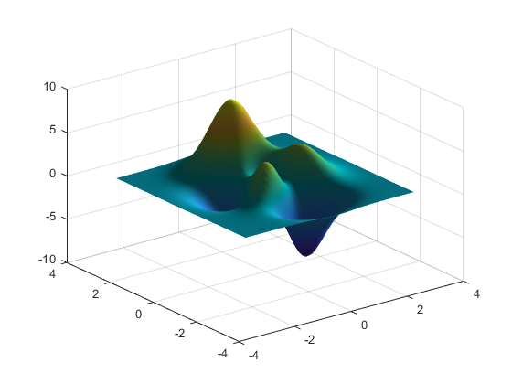
Figure 1: Figure of Merit surface
To plot an analytic function of two parameters it is straightforward to define a structured grid and calculate the output at each point; however, in our framework, each FOM calculation requires a computationally expensive simulation. Sweeping two parameters we could crudely map the FOM, but there is no guarantee that we have resolved important features, as the following figure illustrates.
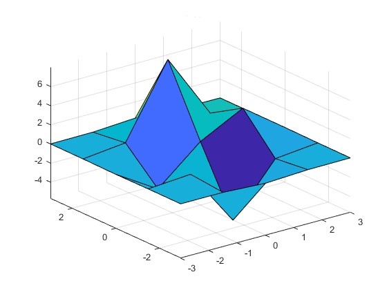
Figure 2: Undersampled parameter space
Ultimately our goal is to find an ‘optimal’ solution, and systematically calculating the surface is unnecessarily expensive; furthermore, this process becomes intractable when the dimension of our space scales up to 10, 100, or 1000s of parameters. If instead, we introduced some overhead to calculate the gradients at each function call, we can determine the next set of parameters more carefully, and in this way, we take a shorter path to find the best solution.
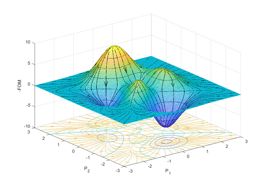
Figure 3: Gradient descent streamlines
Figure 3 illustrates the gradient of the function using streamlines. The optimizer will move in the direction of the streamline, but we have not considered other important factors like step-size or preconditioning. Notice the local minima serve as collectors based on the starting position; yet, some starting positions will not reach these minima such as those along the edge of a ridge. In our implementation, we minimize the FOM, often called the cost function, which is equivalent to maximizing the FOM. For a further discussion on gradient descent methods please see the following articles.
- Gradient Descent: All you Need to Know
- Intro to optimization in deep learning: Gradient Descent
- Scipy Tutorial on Mathematical Optimization
Adjoint Method
Using gradient descent requires finding the partial derivatives with respect to each parameter by varying each individually to get a finite difference approximation of the local derivative. At each step, this results in 1+2N simulations which introduces some overhead but is more efficient than mapping the entire space. It should be noted that once we have an FOM defined we could use any heuristic optimization technique, but at this point, we present some higher mathematics that provides an elegant solution to the problem. Consider the gradient of the FOM with respect to the parameters.
∇pF=(∂F∂p1,⋯,∂F∂pN)
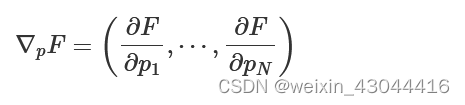
The adjoint state method allows us to efficiently calculate the gradient regardless of the number of parameters. Using integration by parts the original differential equations are recast in terms of the dual space. This has the powerful advantage of requiring only two simulations, forward and adjoint, to calculate the gradient.
In FDTD, the general electromagnetics problem is described by a governing system of linear algebraic equations.
A(p)x=b(p)
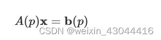
Here A
contains Maxwell's equations, as well as the material permittivity and permeability of the underlying structures at each discretized point in space. The vector x describes all the fields in the simulation region, and b contains the free currents or equivalently the sources. The figure of merit function we have described above, is a function of design parameters, yet a more physically intuitive picture would be to consider F(p)=F(x(p))
.
∂F∂p=∂F∂x∂x∂p
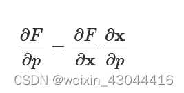
If we find how the FOM varies as a function of the fields and determine the sensitivity of the fields to changes in the parameters we will know the gradient. FDTD will return ∂F/∂x
through the initial forward simulation, but to find how the fields change with each of the parameters ∂x/∂p
we must return to the governing equation. Taking the partial derivative with respect to p, we find the expression.
A∂x∂p=∂b∂p−∂A∂px
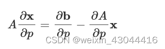
Recall that b is the illumination so ∂b/∂p
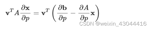
is the change in illumination as the parameters change. The term (∂A/∂p)x can be considered the change to the geometry as a result of changing the parameters. This expression for ∂x/∂p does not actually reduce our costs much, but by introducing a vector vT
the entire equation to reduces to a scaler equality.
vTA∂x∂p=vT(∂b∂p−∂A∂px)
Although, this simplifies the problem we still need to specify this vector vT
. If we require that vTA=∂F/∂x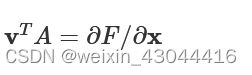
we immediately obtain the quantity of interest, the design sensitivity.
∂F∂p=vT(∂b∂p−∂A∂px)
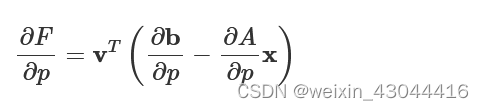
The implication of the above expression is that we can calculate the gradient using exactly two simulations. From the forward simulation, we get the fields, x
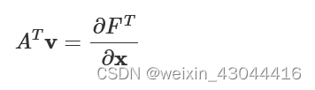
of the simulation volume, which arise due to the defined sources, b, in the presence of an optimizable geometry. We support a figure of merit that is calculated as the power through an aperture projected onto the field profile of a specified mode. In the adjoint simulation, the source is replaced with the adjoint source which takes the place of the FOM monitor. The resulting fields are again recorded everywhere in the optimization region to calculate v
which can be conceptualized as a time-reversal simulation to find the adjoint Maxwell’s equations.
ATv=∂FT∂x
For a more rigorous derivation and further information please see the following excellent resources.
- Adjoint shape optimization applied to electromagnetic design, Optics Express 2013 Vol. 21, Issue 18(2013)
- Optimizing Nanophotonics: from Photorecievers to Waveguides (THESIS), Christopher Lalau-Keraly
Lumopt - Shape vs Topology
This paradigm shift in the design cycle of passive photonic components we often refer to as Inverse Design. For this scheme to work the engineer provides the following:
- Simulation setup
- Parameterization of the design
- Figure of merit
- Reasonable starting point including footprint and materials
Once initialized the optimizer automatically traverses the higher dimensional design space, explores novel designs, and converges on devices with excellent performance. Furthermore, implemented techniques to bound solutions within manufacturable constraints and include performance considerations at process corners.
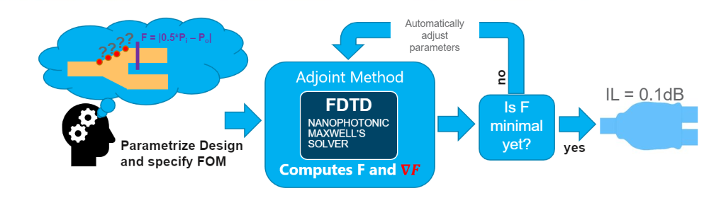
The adjoint methods outlined above are packaged as a python module called lumopt, which uses Lumerical FDTD as a client to solve Maxwell’s equations and scipy libraries to perform the optimization. The initial efforts were undertaken by Christopher Keraly, and this formulation is documented under Lumopt Read the Docs. There are some differences between the version hosted on Github and the lumopt module that ships with the Lumerical installer. We refer to the bundled Lumerical version here exclusively although there are many commonalities. Using this lumopt framework will require a solver license and an API license.
Lumopt comes in two different flavors - shape and topology optimization. With shape optimization one directly defines the geometry parameters to vary, and the bounds of these parameters. For example, the coordinates along the edge of a y-splitter. This allows the user to take a design from a good initial starting point and improve upon it; however, it takes a bit of work to define the geometry and the set of solutions which can be realized with this parameterization may be restrictive. Explicit parameterization like this means that the design rules for manufacturability can be easily enforced.
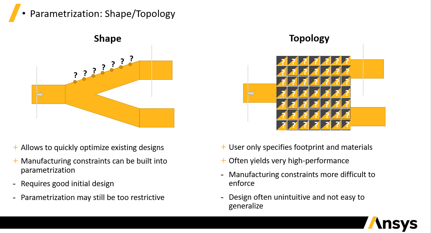
Topological inverse design requires users to simply define an optimizable footprint and the materials involved. As a result, the parameters are simply the voxels of this region which allows for very unintuitive shapes to be realized. Often inexplicably shapes and excellent performance is achieved, yet the structures tend to be harder to fabricate with photolithography owing to the small features that arise. We have taken several measures to ensure their manufacturability including smoothing functions and penalty terms to reduce small features.
For installation and the mechanics of lumopt please see the next section.
Getting Started with lumopt - Python API
Inverse design using lumopt can be run from the CAD script editor, the command line or any python IDE. In the first sub-section, we will briefly describe how to import the lumopt and lumapi modules; although an experienced python user can likely skip this part. As a starting point, it is recommended to run the AppGallery examples and use these as templates for your own project. It may be helpful following along with these files as you read this page or you may simply reference this page when running the examples later. In the project Init section, we outline the project inputs and necessary simulation objects that should be included. Important lumopt specific considerations are highlighted; however, a valid simulation set-up is imperative, so convergence testing should be considered a pre-requisite. Next important lumopt set-up classes, that should be updated to reflect your specifications are documented. Finally, a description of the scipy optimizer and lumopt optimization classes are presented. Shape and topology optimization primarily differ in how they handle the optimizable geometry which is the subject of the next page in this series.
Install
Running from the CAD script editor has the advantage that it requires no set-up and uses a Python 3 distro that ships with the Lumerical installer, so there is no need to install a separate python. This method automatically configures the workspace to find the lumopt and lumapi modules and would be the preferred method for users with little experience in python. Using your own version of python and running from an IDE or the command line may be preferable for more experienced users. To do this one simply needs to import lumopt and lumapi which will require specifying the correct path. Either pass an explicit path using importlibutil, or updating the search path permanently appending the PythonPath object. Advanced user working with numerous libraries might want to create a Lumerical virtual environment. For more information on these methods and os specific paths, see Session management - Python API.
| Note Lumerical ships with a version of Python 3, including lumapi and lumopt modules, already installed. To run any of our examples 'out of the box' simply run the scripts from the script file editor in the CAD. |
Project Init
Base Sim
The base simulation needs to be defined using one of the following options
- Predefined simulation file - Initialize a python variable that specifies the path to the base file. Example Grating coupler.
base_sim = os.path.join(os.path.dirname(__file__), 'grating_base.fsp')
- An lsf set-up script - Create a python variable using the load_from_lsf function. Example Waveguide crossing.
from lumopt.utilities.load_lumerical_scripts import load_from_lsf
crossing_base = load_from_lsf('varFDTD_crossing.lsf')
- Callable python code that does the set-up using the API - This can be a function defined in the same file or an imported function. Example Y-branch.
sys.path.append(os.path.dirname(__file__))  #Add current directory to Python path
from varFDTD_y_branch import y_branch_init_ #Import y_branch_init function from file
y_branch_base = y_branch_init_              #New handle for function
Each method produces a file which the optimizer updates and runs. Since the resulting project files should be equivalent; the method each user employs is a matter of preference or convenience.
Required Objects
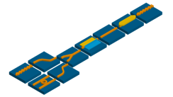
In the varFDTD, and FDTD base simulation it is also necessary to provide input/output geometry and define the following simulation objects that are used by lumopt.
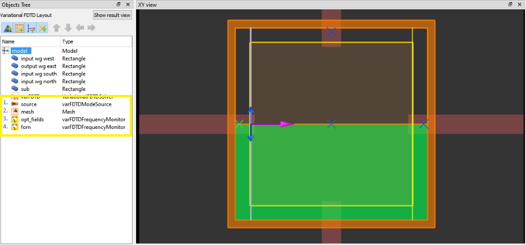
Figure 1: Required simulation inputs
- A mode source - Typically named source, but can be set in the Optimization class.
- A mesh overide region covering the optimization volume - This is a static object, and the pixel/voxel size should be uniform.
- A frequency monitor over the optimization volume - Should be named opt_field, these field values are important for the adjoint method.
- A frequency monitor over the output waveguides - Used to calculate the FOM. The name of this monitor is passed to the ModeMatch class.
The mode source should have a large enough span and the modes should be compared to expectations see FDE convergence. This is used as the forward source. A mesh override is placed over the optimization region to ensure that a fine uniform grid covers this space, and the opt_field monitor is used to extract the fields in this region. The FOM monitor should be aligned to the interface of a mesh cell to avoid interpolation errors; therefore, it is a good idea to have a mesh override co-located with the FOM monitor. In the adjoint simulation, the adjoint source will take the place of the FOM monitor. Passing the name of the FOM monitor, to modematch class, allows multiple FOM monitors to be defined in the same base file which is helpful for SuperOptimization.
Set-up Classes
Two important lumopt classes that should be updated with your parameters are wavelengths and modematch. These are used to define the spectrum and mode number(or polarization) of the FOM respectively. It should be noted here that the FOM we accept is power coupling of guided modes. Other figures of merit, such as optimizing the target phase or power to a specified grating order are not supported. To compute the broadband figure of merit we take the mean of the target minus the error using the p-norm.
F=(1λ2−λ1∫λ2λ1|T0(λ)|pdλ)1/p−(1λ2−λ1∫λ2λ1|T(λ)−T0(λ)|pdλ)1/p
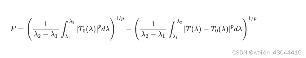
where
- T0
- is the target_T_fwd
- λ1 and λ2
- are the lower and upper limits of the wavelength points
- T
- is the actual mode expansion power transmission
- p
- is the value of the generalized p-norm
Wavelengths
Defines the simulation bandwidth, and wavelength resolution. Defining the target FOM spectrum is done in modematch.
from lumopt.utilities.wavelengths import Wavelengths
class Wavelengths(start,
                  stop,
                  points)
: start: float
Shortest wavelength [m]
: stop: float
Longest wavelength [m]
: points: int
The number of points, uniformly spaced including the endpoints.
Example
wavelengths = Wavelengths(start = 1260e-9, stop = 1360e-9, points = 11)
ModeMatch
This class is used to define target mode, propagation direction, and specify the broadband power coupling.
from lumopt.figures_of_merit.modematch import ModeMatch
class ModeMatch(monitor_name,
                mode_number,
                direction,
                target_T_fwd,
                norm_p,
                target_fom)
: monitor_name: str
Name of the FOM monitor in the file.
: mode_number : str or int
Used to specify the mode.
If the varFDTD solver is used:
- ‘fundamental mode’
- int - user select mode number
If the FDTD solver is used:
- 'fundamental mode'
- 'fundamental TE mode'
- 'fundamental TM mode'
- int - user select mode number
: direction : str
The direction is determined by the FDTD coordinates; for mode traveling in the positive direction the direction is forward.
- 'Backward'
- 'Forward'
: multi_freq_source: boolean, optional
Should only be enabled by advanced users. See frequency Frequency dependent mode profile for more info. Default = False
: target_T_fwd: float or function
A function which will take the number of Wavelengths points and return values [0,1]. Usually passed as a lambda function or a single float value for single wavelength FOM. To specify a more advanced spectrum one can define a function, it may be helpful to use, numpy windows as a template.
: norm_p: float
Is the generalized p-norm used in the FOM calculation. The p-norm, with p≥1
allows the user to increase the weight of the error. Since p=1
provides a lower bound on this function, a higher p-number will increase the weight of the error term. Default p =1.0
: target_fom: float
A target value for the figure of merit. This will change the behavior of the printing and plotting only. If this is enabled, by setting a value other than 0.0, the distance of the current FOM is given. Default = 0.0
Example
class ModeMatch(monitor_name = 'fom', mode_number = 3, direction = 'Backward', target_T_fwd = lambda wl: np.ones(wl.size), norm_p = 1)
Optimization Classes
Here we describe the generic ScipyOptimizer wrapper, and lumopt Optimization class which is used to encapsulate the project.
ScipyOptimizer
This is a wrapper for the generic and powerful SciPy optimization package.
from lumopt.optimizers.generic_optimizers import ScipyOptimizers
Class ScipyOptimizers(max_iter,
                      method,
                      scaling_factor,
                      pgtol,
                      ftol,
                      scale_initial_gradient_to,
                      penalty_fun,
                      penalty_jac)
: max_iter: int
Maximum number of iterations; each iteration can make multiple figure of merit and gradient evaluations. Default = 100
: method: str
Chosen minimization algorithm; experimenting with this option should only be done by advanced users. Default = ‘L-BFGS-B'
: scaling_factor: none, float, np.array
None, scalar or a vector the same length as the optimization parameters. This is used to scale the optimization parameters. As of 2021R1.1, the default behavior in shape optimization is to automatically map the parameters the range [0,1] within the optimization routines; which was always the case in topology. The bounds, defined in the geometry class, or eps_min/eps_max are used for this. Default = None
: pgtol: float
The iteration will stop when max(|proj gi| i = 1, ..., n)<=pgtol|![]()
where gi
is the i-th component of the projected gradient. Default = 1.0e-5
: ftol: float
The iteration stops when ((fk−fk+1)/max(|fk| , |fk+1| , 1))<=ftol
. Default = 1.0e-5

: scale_initial_gradient_to: float
Enforces a rescaling of the gradient to change the optimization parameters by at least this much; the default value of zero disables automatic scaling. Default = 0.0
: penalty_fun: function, optional
Penalty function to be added to the figure of merit; it must be a function that takes a vector with the optimization parameters and returns a single value. Advanced feature. Default = None
:penalty_jac: function, optional
The gradient of the penalty function; must be a function that takes a vector with the optimization parameters and returns a vector of the same length. If a penalty_fun is included with no penalty_jac, lumopt will approximate the derivative. Advanced feature. Default = None
Example
optimizer = ScipyOptimizers(max_iter = 200,
                            method = 'L-BFGS-B',
                            scaling_factor = 1.0,
                            pgtol = 1.0e-5,
                            ftol = 1.0e-5,
                            scale_initial_gradient_to = 0.0,
                            penalty_fun = penalty_fun,
                            penalty_jac = None)
Optimization
Encapuslates and orchestrates all of the optimization pieces, and routines. Calling the opt.run method will perform the optimization.
from lumopt.optimization import Optimization
class Optimization(base_script,
                   wavelengths,
                   fom,
                   geometry,
                   optimizer,
                   use_var_fdtd,
                   hide_fdtd_cad,
                   use_deps,
                   plot_history,
                   store_all_simulations,
                   save_global_index,
                   label,
                   source_name)
: base_script: callable, or str
Base simulation - See project init.
- Python function in the workspace
- String that points to base file
- Variable that loads from lsf script
: wavelengths: float or class Wavelengths
Provides the optimization bandwidth. Float value for single wavelength optimization and Wavelengths class provides a broadband spectral range for all simulations.
: fom: class ModeMatch
The figure of merit FOM, see ModeMatch
: geometry: Lumopt geometry class
This defines the optimizable geometry, see Optimizeable Geometry
: optimizer: class ScipyOptimizers
See ScipyOptimizer for more information.
: hide_fdtd_cad: bool
Flag to run FDTD CAD in the background. Default = False
: use_deps: bool
Flag to use the numerical derivatives calculated directly from FDTD. Default = True
: plot_history: bool
Plot the history of all parameters (and gradients). Default = True
: store_all_simulations: bool
Indicates if the project file for each iteration should be stored or not. Default = True
: save_global_index: bool
Flag to save the results from a global index monitor to file after each iteration (used for visualization purposes). Default = False
: label: str, optional
If the optimization is part of a super-optimization, this string is used for the legend of the corresponding FOM plot. Default = None
: source_name: str, optional
Name of the source object in the simulation project. Default = "source"
Example
 opt_2d = Optimization(base_script = base_sim_2d,
                       wavelengths = wavelengths,
                       fom = fom,
                       geometry = geometry,
                       optimizer = optimizer,
                       use_var_fdtd = False,
                       hide_fdtd_cad = True,
                       use_deps = True,
                       plot_history = True,
                       store_all_simulations = True,
                       save_global_index = False,
                       label = None)
Note(Advanced): For 2020R2 we exposed, a prototype user-requested debugging function that allows the user to perform checks of the gradient calculation. This is a method of the optimization class and can be called as follows.
opt.check_gradient(intitial_guess, dx=1e-3)
Where initial_guess is a numpy array that specifies the optimization parameters at which the gradient should be checked. The scalar parameter dx is used for the central finite difference approximation
Has two limitations; one the check performs an unnecessary adjoint simulation. Two the check_gradient is only available for regular optimizations and not superoptimizations of multiple FOMs.
Superoptimization
The + operator has been overloaded in the optimization class so it is trivial to simultaneously optimize:
- Different output waveguides and\or wavelength bands CWDM
- Ensure balanced TE\TM performance or suppress one over the other
- Robust manufacturing by simultaneously optimizing underetch\overtech\nominal variations.
- Etc ...
Simply adds the various Optimization classes together to create a new SuperOptimization object. Then you will call run on this object to co-optimize the various optimization definitions. Each FOM calculation requires 1 optimization object so the number of simulations at each iteration will be Nsim=2×NFOM
.
Example
 opt = opt_TE + opt_TM
 opt.run(working_dir = working_dir)
Optimizable Geometry - Python API
This section covers the details of shape and topology based inverse design using lumopt. As prerequisite please familiarize yourself with photonic inverse design and understand the basics of the lumopt workflow.
The following examples can help provide context to the information presented here.
Shape
Shape based optimization allows users to take strong existing designs and improve their performance. Constraints can be easily included in the parameterization such as design rules for manufacturing. To do this the user needs to parameterize their geometry, through a shape function s(p)
and provide bounds on the p values. This is supported with a handful of geometry classes FunctionDefinedPolygon which accepts a python function of parameters, and ParamterizedGeometry which accepts a python API function. FDTD is used to calculate the FOM(s(p))
.
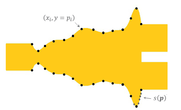
Figure 1: Shape parameters and the shape function
The Adjoint method motivation section described how the parameters enter the equations through the permittivity. When users define a parameterized geometry an additional step, we refer to as the d_eps_calculation, is required to determine how varying each parameter changes the permittivity in Maxwell’s equations and the subsequent shape derivative. This is accomplished by meshing the simulation and returning the ϵ(x,y,z)
, but without running the solver. Since this must be done for each parameter, including more parameters comes at some extra cost; although, this should be small compared to running the simulation; however, in large 3D simulations this meshing step can be intensive even if it is brief. If you need assistance improving the performance, and parallelization of the d_eps calculation please reach out to Lumerical support. For more information on the shape derivative approximation method see Chpt 5 of Owen Miller's thesis.
It is important to consider that the choice of parameters may be too restrictive, and that gradient based techniques are inherently dependent on initial conditions. It not always obvious what a better choice of parameters and initial conditions may be so some experimentation may be required to achieve the greatest performance.
Shape Geometry Classes
For each geometry class the user must pass the shape function, parameter bounds, geometry specifications and material properties. It is important to verify that your geometry varies smoothly and does not self-intersect for any combination of acceptable parameters as this can produce discontinuities in the gradient calculation. Spline points are not bounded in the same way the parameters are which can be problematic. When end points are clamped this may lead to discontinuities, employing "not-a-knot spline" usually avoids these errors. By visualizing different shapes realized from possible sets of bounded parameters most of these errors can be recognized and avoided.
Functiondefinedpolygon
This python class takes a user defined function of the optimization parameters. The function defines a polygon by returning a set of vertices, as a numpy array of coordinate pairs np.array([(x0,y0),…,(xn,yn)]), where the vertices must be ordered in a counter-clockwise direction.
from lumopt.geometries.polygon import FunctionDefinedPolygon
class  FunctionDefinedPolygon(func,
                              initial_params,
                              bounds,
                              z,
                              depth,
                              eps_out,
                              eps_in,
                              edge_precision,
                              dx,
                              deps_num_threads)
: func : function
function(parameters) - Returns s(p)
an np.array([(x0,y0),…,(xn,yn)]) of coordinate tuples ordered CCW.
Typically, a subset of polygon points p
will be used as parameters with a spline technique to up-sample these values and create a smoother curve. This user defined function is a common source of error.
: initial_params: np.array
Parameters in a form accepted by the func, that define the initial geometry. Size = [1, n_param]
: bounds: np.array
A set of tuples that define the min and max of each parameter. Size = [2, n_param]
: z : float
Center of polygon along the z-axis. Default = 0.0
: depth: float
Span of polygon along the z-axis.
: eps_out: float
permittivity of the material around the polygon.
: eps_in: float
Permittivity of the polygon material.
: edge_precision: int
Number of quadrature points along each edge for computing the FOM gradient using the shape derivative approximation method.
: dx: float > 0.0
Step size for computing the FOM gradient using permittivity perturbations. Default = 1e-5
: deps_num_threads: int, optional
Number of threads to be uses in the d_eps calculation. This utilizes the job manager, and changes your resource configuration. By default this will be performed serially, but it is possible to utilize more cores simultaneously by setting this greater than 1. This is an advanced, experimental feature with some some additional overhead associated; thus, testing and benchmarking is required. In the event of an unexpected termination one will have to manually fix the update. Resource configuration elements and controls. Default = 1
ParameterizedGeometry
from lumopt.geometries.parameterized_geometry import ParameterizedGeometry
class ParameterizedGeometry(func,
                            initial_params,
                            bounds,
                            dx,
                            deps_num_threads)
: func : python API function
function(parameters, fdtd, only_update, (optional arguments))
This function is less concise, but more intuitive and flexible than FunctionDefinePolygon. It allows users to call the API methods, in the same way you would use lsf script commands to set-up and update the geometry rather than passing the (x,y) vertices. The flag 'only_update' is used to avoid frequent recreations of the parameterized geometry which reduces the performance. When the flag is true, it is assumed that the geometry was already added at least once to the CAD. For an example of it's usage see Inverse design of grating coupler.
: initial_params: np.array
Parameters in a form accepted by the func, that define the initial geometry. Size = [1, n_param]
: bounds: np.array
A set of tuples that define the min and max of each parameter. Size = [2, n_param]
: dx: float > 0.0
Step size for computing the FOM gradient using permittivity perturbations. Default = 1e-5
: deps_num_threads: int, optional
Number of threads to be uses in the d_eps calculation. This utilizes the job manager, and changes your resource configuration. By default this will be performed serially, but it is possible to utilize more cores simultaneously by setting this greater than 1. This is an advanced, experimental feature with some some additional overhead associated; thus, testing and benchmarking is required. In the event of an unexpected termination one will have to manually fix the update. Resource configuration elements and controls. Default = 1
Shape Considerations
From 2D to 3D
Shape optimization in 2D is supported through MODE varFDTD and FDTD. Using varFDTD will automatically collapse the material and geometric contributions in the z-direction to more accurately reflect the effective indices. FDTD simply uses the material index, ignoring the 3rd dimension. For in-plane integrated photonic components varFDTD provides the most straightforward route to accurate permittivity values. One can use FDTD in this situation as well, but determining the effective indices is up to the user. In situations where the propagation is not entirely in plane, such as with the grating coupler example, FDTD is required. To use varFDTD set the use_varFDTD = True in the optimization class.
In shape optimization it is straightforward to move from 2D to 3D since all the supported geometry classes are transferable. The only update required is to change the base file monitors and simulation region from 2D to 3D FDTD. Bulk material indices should be specified for eps_in and eps_out as the geometric contributions are automatically incorporated into the update equations. We have found strong correlation between high performing devices in 2D and device performance in 3D; however, expect the FOM to be reduced when moving to 3D as new loss mechanisms are considered. Due to the complexity and time required for 3D optimizations we recommend starting in 2D and then importing those optimized structures into 3D for a final abbreviated optimization run.
GDS Export
When exporting the optimized geometry we recommend using the encrypted GDS export script, outlined and available for download here:
Topology
In topology optimization the user does not need to parameterize the geometry, which simplifies the workflow; however, the simulation needs to perform a few more complicated steps to produce physically realizable devices. To set up topology optimization simply define the optimizable footprint and materials in the relevant 2D or 3D geometry class, outline below. Each FDTD mesh cell in the discretized optimization volume becomes a parameter. This technique often scales to thousands of parameters, but with the adjoint method we still only need 2 simulations per iteration to calculate the gradient. Furthermore, since the permittivity values are the optimization parameters, there is a direct link to Maxwell’s equations so there is no need to perform a d_eps as calculation.
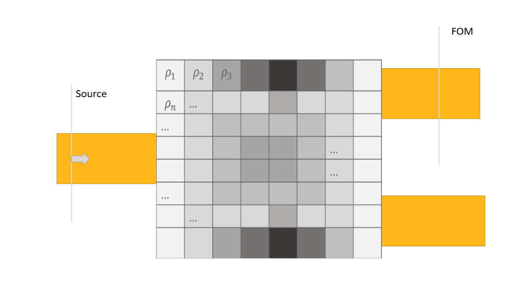
Figure 2: Topology optimization schematic
In the initialization section we describe important aspects of the setup, and how to provide initial conditions. Once the optimization is running it proceeds in two or three steps. First the greyscale phase where the parameters vary continuously between the core and cladding index. Next, a binarization phase is run to force the mesh cells to take either the core or cladding index. Finally, an optional design for manufacturing step is implemented. In this step a penalty function is added to the FOM. The magnitude of the penalty function is determined by the degree to which the minimum feature size constraint is violated. Finally, we will discuss how to move from 2D to 3D, and export your designs to GDS .
Topology Geometry Classes
TopologyOptimization2D
This class is used in 2D simulations.
from lumopt.geometries.topology import TopologyOptimization2D
class TopologyOptimization2D(params,
                             eps_min,
                             eps_max,
                             x, y, z,
                             filter_R,
                             eta,
                             beta,
                             min_feature_size)
: params : np.array
Initial parameters that define the initial geometry. Size = [n_x, n_y]
: eps_min : float
Permittivity of the core material
: eps_max: float
Permittivity of the cladding
: x: np.array
The x position of the parameters and FDTD unit cells in [m].
: y : np.array
The y positions of the parameters and FDTD unit cells in [m].
: z : float
Z position of the topology object in [m]. Default 0.0
: filter_R: float
The radius of the Heaviside filter in [m]. Outlined in greyscale. Default = 200e-9
: eta : float
Eta parameter of the Heaviside filter. Provides a shift of the binarization threshold towards eps_min if eta <0.5, and towards eps_max if eta >0.5. Default = 0.5
: beta: float
Beta parameter of the Heaviside filter. This is the starting value used, but the beta parameter is ramped up to ~1000 during the binarization phase. Default = 1
: min_feature_size: float, optional
Minimum feature size in the DFM phase. Features smaller than this value will be penalized in the final DFM stage. Must be filter_R < min_feature_size < 2.0 * filter_R. A value of 0.0 will disable the DFM phase. Default = 0.0
TopologyOptimization3DLayered
This class is used in 3D simulations, and operates in the same way as the 2D geometry with the exception that z is now a required nump array of points, and the optimization region is a volume. To reduce the field results to the XY plane there is an integration along z. The pattern of the layer is optimized for, but not each mesh cell individually: ie it is not a full 3D voxelated topological geometry, that feature is currently not supported.
from lumopt.geometries.topology import TopologyOptimization3DLayered
class TopologyOptimization3DLayered(params,
                                    eps_min,
                                    eps_max,
                                    x, y, z,
                                    filter_R,
                                    eta,
                                    beta,
                                    min_feature_size)
: params : np.array
Initial parameters that define the initial geometry. Size = [n_x, n_y, n_z]
: eps_min : float
Permittivity of the cladding
: eps_max: float
Permittivity of the core material
: x: np.array
The x position of the parameters and FDTD unit cells in [m].
: y : np.array
The y positions of the parameters and FDTD unit cells in [m].
: z : np.array
The z position of the parameters and FDTD unit cells in [m].
: filter_R: float
The radius of the Heaviside filter in [m]. Outlined in greyscale. Default = 200e-9
: eta : float
Eta parameter of the Heaviside filter. Provides a shift of the binarization threshold towards eps_min if eta <0.5, and towards eps_max if eta >0.5. Default = 0.5
: beta: float
Beta parameter of the Heaviside filter. This is the starting value used, but the beta parameter is ramped up to ~1000 during the binarization phase. Default = 1
: min_feature_size: float, optional
Minimum feature size in the DFM phase. Features smaller than this value will be penalized in the final DFM stage. Must be filter_R < min_feature_size < 2.0 * filter_R. A value of 0.0 will disable the DFM phase. Default = 0.0
Running
This is section describes the various stages of topology optimization.
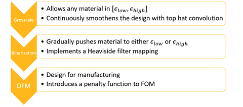
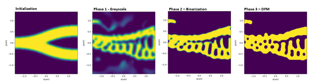
Figure 3: Topology optimization steps
Initialization
It is important the mesh defined in the FDTD simulation precisely matches the optimization parameters defined in Python. To do this make sure a uniform mesh is defined over the optimizable footprint. The python parameters may be defined as follows.
#Footprint and pixel size
size_x = 3000        #< Length of the device (in nm). Longer devices typically lead to better performance
delta_x = 25        #< Size of a pixel along x-axis (in nm)
size_y = 3000        #<Extent along the y-axis (in nm). When using symmetry this should half the size.
delta_y = 25        #< Size of a pixel along y-axis (in nm)
size_z = 240        #< Size of device in z direction
delta_z = 40        #< Size of a pixel along z-axis (in nm)

x_points=int(size_x/delta_x)+1
y_points=int(size_y/delta_y)+1
z_points=int(size_z/delta_z)+1

#Convert to SI position vectors
x_pos = np.linspace(-size_x/2,size_x/2,x_points)*1e-9
y_pos = np.linspace(-size_y/2,size_y/2,y_points)*1e-9
z_pos = np.linspace(-size_z/2,size_z/2,z_points)*1e-9
In the lumerical script that generates the base file ensure that the grid matches. Alternative methods such as a python function or base file are also allowed, but the grid and parameter values will also need to match.
#Define footprint
opt_size_x=3e-6;
opt_size_y=3e-6;
opt_size_z=240e-9;

#Define pixel size
dx = 25e-9;
dy = 25e-9;
dz = 40e-9;

addmesh;
set('name','opt_fields_mesh');
set('override x mesh',true);  set('dx',dx);
set('override y mesh',true); set('dy',dy);
set('override z mesh',true); set('dy',dz);
set('x',0); set('x span',opt_size_x);
set('y',0); set('y span',opt_size_y);
set('z',0); set('z span',opt_size_z);
To set the initial conditions you can pass an np.array the same size as the parameters. If you want start with a uniform permittivity value across the optimizable domain this is straightforward.
##Initial conditions
#initial_cond = np.ones((x_points,y_points))       #< Start with the domain filled with eps_max
#initial_cond = 0.5*np.ones((x_points,y_points))   #< Start with the domain filled with (eps_max+eps_min)/2
#initial_cond = np.zeros((x_points,y_points))      #< Start with the domain filled with eps_min
Alternatively, define an initial structure in the base simulation, and pass None. In this case the optimizer meshes the simulation to determine the initial parameter set. This should be a structure group containing the relevant geometry called initial_guess.
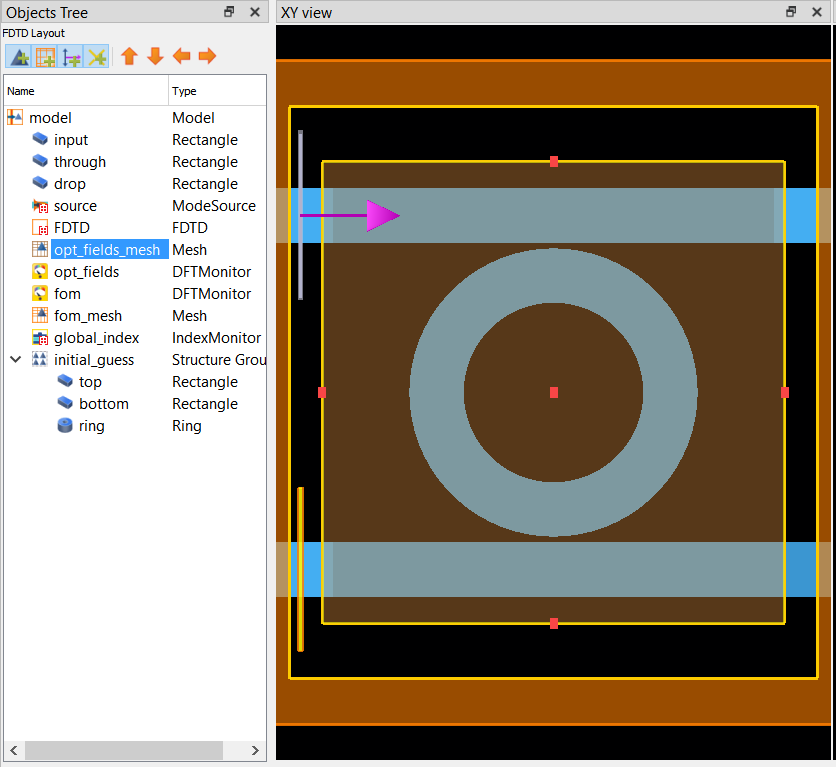
Figure 4: Topology optimization set-up
Greyscale
In the python optimization each cell corresponds to a parameter ρ∈[0,1]
which is linearly mapped to the ϵ
values in FDTD. A circular top hat convolution with a user specified radius is used to remove sharp corner, small holes or islands which can’t be manufactured through convolution. Depending on you manufacturing process, typical values for the filter radius will be between 50 and 500nm.
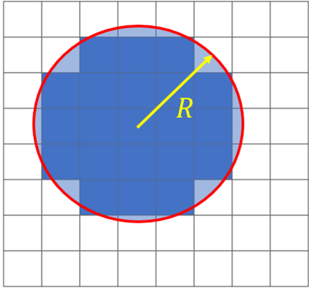
Figure 5: Top-hat convolution diagram
In this stage of the optimization the FOM error tends to very quickly reduce but may take 100’s of iterations to reach a minima. The values obtained during greyscale are typically very good, but the filtering process is imperfect, and there will be intermediate eps values and unproducible features via lithographic means. The following steps are used to produce realizable devices.
Binarization
During binarization the Heaviside filter changes the mapping of the python elements to FDTD permittivity. In the greyscale phase the beta parameter is 1, producing a linear mapping. During binarization the beta parameter is incrementally ramped up. The Heaviside filter is defined as follows, and ramping up the beta parameter converts it from a linear mapping to a step function.
ϵi=ϵlow+tanh(βη)+tanh(β(ρi−η))tanh(βη)+tanh(β(1−η))Δϵ
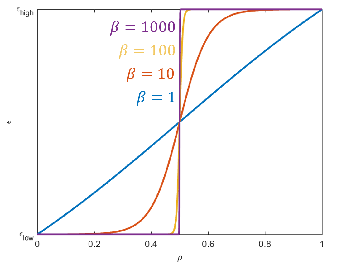
Figure 6: Heaviside filter
Ramping β
up will perturbs the system producing sharp peaks in the FOM. It is followed by a set of optimization iterations to adjust to the perturbation, and reduce the FOM error. It is possible to change the number of iterations between increments of Beta, by changing the opt.continuation_max parameter.
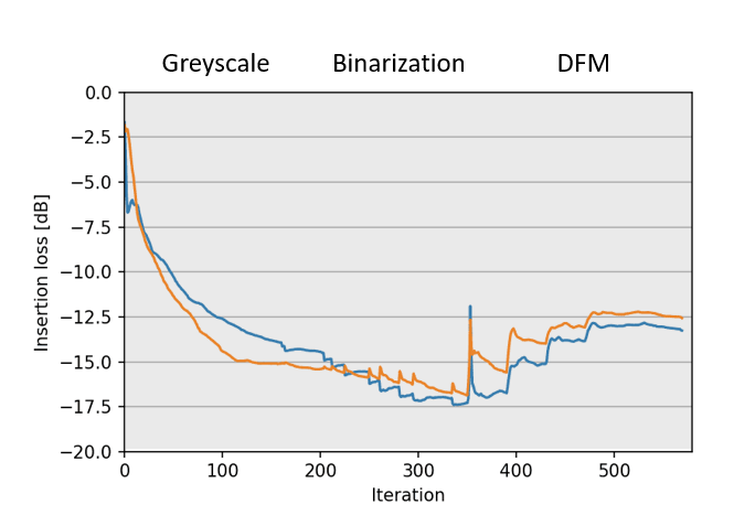
Figure 7: FOM during optimization steps
Design For Manufacturing (optional)
Even when using the Heaviside filter for spatial filtering, the topology optimization designs tend to create features that break process design rules. To ensure manufacturability we explored ways of explicitly enforcing specific minimum feature size constraints. Our implementation uses a technique published by Zhou et al. in 2015[1]. This paper was focused structural mechanics, so we had to make some small adjustments to make it work reliably for photonic devices.
The main idea is to come up with an indicator function which is minimal if the minimum feature size constraints are fulfilled everywhere. This term is then added as a penalty term to the FOM during optimization. To implement this phase pass a non-zero min_feature_size constraint to the geometry class.
Topology Considerations
From 2D to 3D
All dimensional considerations from shape apply to topology. We recommend using effective indices as calculated in varFDTD as the permittivity values in 2D opt, but one should work with FDTD for all topology optimizations.
When going from 2D to 3D in topology the performance does not correlate as well, as in shape based designs. That being said good 2D results demonstrate the possibility of producing strong 3D designs which is important. Performance improvements in 3D tend to proceed more quickly if one imports a design that is not fully binarized, which relaxes the abillity of the 3D optimizer to vary parameters. Importing partially binarized 2D designs into 3D is outlined below.
## First, we specify in which path to find the 2d optimization
path2d = os.path.join(cur_path,"[Name of 2D opt folder]")

## Next, check the log-file to figure out which iteration we should load from.
# It is usually best to load something mid-way through the binarization
convergence_data = np.genfromtxt(os.path.join(path2d, 'convergence_report.txt'), delimiter=',')

## Find the first row where the beta value (3rd column) is larger than beta_threshold (here 10)
beta_threshold = 10
beta_filter = convergence_data[:,2]>beta_threshold
convergence_data = convergence_data[beta_filter,:]  #< Trim data down
iteration_number = int(convergence_data[0,0]-2)

## Load the 2d parameter file for the specified iteration
geom2d = TopologyOptimization2D.from_file(os.path.join(path2d, 'parameters_{}.npz'.format(iteration_number) ), filter_R=filter_R, eta=0.5)
startingParams = geom2d.last_params     #< Use the loaded parameters as starting parameters for 3d
startingBeta   = geom2d.beta            #< Also start with the same beta value. One could start with 1 as well.
Export to GDS
Since the topology designed devices do not have a well defined shape we developed an alternate method to extract the GDSII designs using contours. This functionality is outlined in the following KX page.
Further Resources
Webinars
- Feb 2019 - Broadband shape
- Aug 2019 - Updates to Shape, Grating Couplers, and Intro to Topology Optimization
- April 2020 - Update to Topology Optimization
Examples
- GDS Pattern Extraction Using getcontours
- Inverse Design of an Efficient Narrowband Grating Coupler
- Broadband Grating Coupler Design Bandwidth vs Peak Efficiency
- Inverse Design of a Y-Splitter using Topology Optimization
- Topology Optimization of an O,C Band Splitter with min_feature_size Constraint
References
Application Examples
Using the Python API in the nanowire application example

This example demonstrates the feasibility of integrating Lumerical FDTD with Python using Application Programming Interface (API). In this example, we will set the geometry based on 2D Mie scattering example and then run the simulation using Python script. Once the simulation is finished, simulation results will be imported to Python, and plots comparing simulation and theoretical results as well as a plot of Ey intensity will be provided.
Requirements: Lumerical products 2018a R4 or newer
Note:
- Versions : The example files were created using Lumerical 2018a R4, Python 3.6 (and numpy), matplotlib 0.99.1.1, and Windows 7
- Working directory : It should be possible to store the files in any locations as desired. However, it is recommended to put the Lumerical and Python files in the same folder in order for the above script files to work properly. It is also important to check the Lumerical working directory has the correct path, see here for instructions to change the Lumerical working directory.
- Linux: /opt/lumerical/interconnect/api/python/
- Windows: C:\Program Files\Lumerical\FDTD\api\python
During the Lumerical product installation process, a lumapi.py file should be automatically installed in this location.
This module is the key to enable Lumerical-Python API connection. Once the lumapi module is imported to Python, the integration should be ready. See this page for instructions for setting up Python API.
Note: Running Lumerical files from Python
If you already have the FDTD simulation or script files ready, you can run them from Python. For example, download the Lumerical script files ( nanowire_build_script.lsf and nanowire_plotcs.lsf ) and the nanowire_theory.csv text file and then run the script commands below in Python:
import lumapi
nw = lumapi.FDTD("nanowire_build_script.lsf")
nw.save("nanowire_test")
nw.run()
nw.feval("nanowire_plotcs.lsf")  # run the second script for plots
The commands above run the nanowire_build_script.lsf to set the geometry first, and then runs nanowire_plotcs.lsf to plot the simulation and theoretical results. These plots are created using Lumerical visualizer and will be identical to the plots in nanowire application example . In the rest of this page an explanation on how to build the geometry and analyze the results directly from Python will be provided.
Importing modules
The following script lines imports the modules ( importlib.util , numpy and matplotlib ) and the Lumerical Python API that will be used in the later script.
import importlib.util
#The default paths for windows
spec_win = importlib.util.spec_from_file_location('lumapi', 'C:\\Program Files\\Lumerical\\2020a\\api\\python\\lumapi.py')
#Functions that perform the actual loading
lumapi = importlib.util.module_from_spec(spec_win) #
spec.loader.exec_module(lumapi)
import numpy as np
import matplotlib.pyplot as plt
User can also use the method mentioned in the session management
Setting up the geometry from Python
The cross section results are wavelength dependent. To obtain the field profile for resonant mode we need to run two simulations: first simulation to calculate the resonance wavelength, and second simulation to adjust the wavelength of the profile monitor accordingly. Therefore, we define a function that sets the geometry and has profile monitor wavelength as an argument:
def runNanowireSimulation(profile_monitor_wavelength=1e-6):
    configuration = (
        ("source", (("polarization angle", 0.),
                    ("injection axis", "y"),
                    ("x", 0.),
                    ("y", 0.),
                    ("x span", 100.0e-9),
                    ("y span", 100.0e-9),
                    ("wavelength start", 300.0e-9),
                    ("wavelength stop", 400.0e-9))),
        #see attached file for complete configuration
   )
To set the geometry, we found that it is more efficient and cleaner to use nested tuple, however, advanced users may use any ordered collection. The order is important if a property depends on the value of another property.
    for obj, parameters in configuration:
       for k, v in parameters:
           fdtd.setnamed(obj, k, v)

    fdtd.setnamed("profile", "wavelength center", float(profile_monitor_wavelength))
    fdtd.setglobalmonitor("frequency points", 100.) # setting the global frequency resolution
    fdtd.save("nanowire_test")
    fdtd.run()
    return fdtd.getresult("scat", "sigma"), fdtd.getresult("total", "sigma"), fdtd.getresult("profile", "E")
Analyzing simulation and theoretical results
The script then calls the function to run the simulation, and then imports the simulation results into Python. Theoretical results are also imported from the nanowire_theory.csv file and interpolated over the simulation wavelengths:
nw = runNanowireSimulation() # recalls the function to run the simulation

## run the simulation once, to determine resonance wavelength
## and get cross-sections from analysis objects
sigmascat, sigmaabs, _ = runNanowireSimulation()
lam_sim = sigmascat['lambda'][:,0]
f_sim = sigmascat['f'][:,0]
sigmascat = sigmascat['sigma']
sigmaabs  = sigmaabs['sigma']
sigmaext = -sigmaabs + sigmascat

#load cross section theory from .csv file
nw_theory=np.genfromtxt("nanowire_theory.csv", delimiter=",")
nw_theory.shape
lam_theory = nw_theory[:,0]*1.e-9
r23 = nw_theory[:,1:4]*2*23*1e-9
r24 = nw_theory[:,4:7]*2*24*1e-9
r25 = nw_theory[:,7:10]*2*25*1e-9
r26 = nw_theory[:,10:13]*2*26*1e-9
r27 = nw_theory[:,13:16]*2*27*1e-9

for i in range(0,3):  # interpolate theoretical data
    r23[:,i] = np.interp(lam_sim,lam_theory,r23[:,i])
    r24[:,i] = np.interp(lam_sim,lam_theory,r24[:,i])
    r25[:,i] = np.interp(lam_sim,lam_theory,r25[:,i])
    r26[:,i] = np.interp(lam_sim,lam_theory,r26[:,i])
    r27[:,i] = np.interp(lam_sim,lam_theory,r27[:,i])
Plotting the results
One of the benefits of using the Lumerical Python API is that we can take advantage of the advanced Python modules. In this example, we use pyplot in the matplotlib module to plot the results.
The following commands plot the simulation and theoretical results for comparison.
plt.plot(lam_sim*1e9, sigmaext*1e9,label='sigmaext')
plt.plot(lam_sim*1e9, -sigmaabs*1e9)
plt.plot(lam_sim*1e9, sigmascat*1e9)
plt.plot(lam_sim*1e9, r25*1e9)
plt.xlabel('wavelength (nm)')
plt.ylabel('cross section (nm)')
plt.legend(['Extinction','Absorption', 'Scattering', 'r25 theory', 'r25 theory',
            'r25 theory'])
plt.show()

plt.plot(lam_sim*1e9, sigmaext*1e9,label='sigmaext')
plt.plot(lam_sim*1e9, -sigmaabs*1e9)
plt.plot(lam_sim*1e9, sigmascat*1e9)
plt.plot(lam_sim*1e9, r24*1e9)
plt.plot(lam_sim*1e9, r26*1e9)
plt.xlabel('wavelength (nm)')
plt.ylabel('cross section (nm)')
plt.legend(['Extinction','Absorption', 'Scattering', 'r24 theory', 'r24 theory',
            'r24 theory', 'r26 theory', 'r26 theory','r26 theory'])

plt.show()
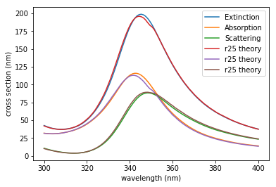
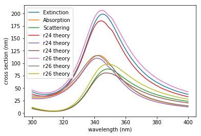
The above plots shows that the maximum extinction occurs near 348nm. This can be achieved by using numpy.argmax . To show the field profile at this wavelength, the wavelength of the profile monitor is adjusted and simulation is re-run for the second time using the commands below:
## run the simulation again using the resonance wavelength
_, _, E = runNanowireSimulation(profile_monitor_wavelength=lam_sim[np.argmax(sigmascat)])

## show the field intensity profile
Ey = E["E"][:,:,0,0,1]
Once the simulation is finished, we can extract the profile monitor results and plot |Ey|^2 at z=0:
  plt.pcolor(np.transpose(abs(Ey)**2), vmax=5, vmin=0)
  plt.xlabel("x (nm)")
  plt.ylabel("y (nm)")
  plt.xticks(range(Ey.shape[0])[::25], [int(v) for v in E["x"][:,0][::25]*1e9])
  plt.yticks(range(Ey.shape[1])[::25], [int(v) for v in E["y"][:,0][::25]*1e9])
  plt.colorbar()
  plt.show()
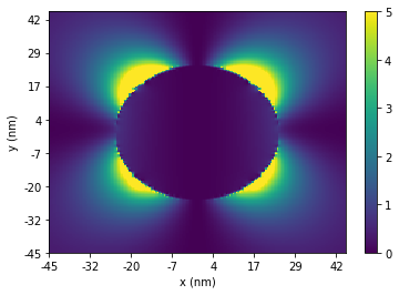
Inverse Design of Grating Coupler (2D)
FDTD MODE Automation API Gratings Inverse design / Optimization Photonic Integrated Circuits - Passive
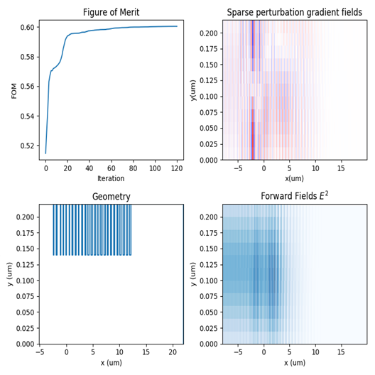
In this example, we will use the Inverse Design toolbox (lumopt) to design a silicon-on-insulator (SOI) grating coupler. Compared to other optimization methods such as particle swarm optimization (PSO), this optimization algorithm enables obtaining the best solution in just a few iterations. The optimum design will be exported into a GDS file for further simulation and/or fabrication.
Overview
Understand the simulation workflow and key results
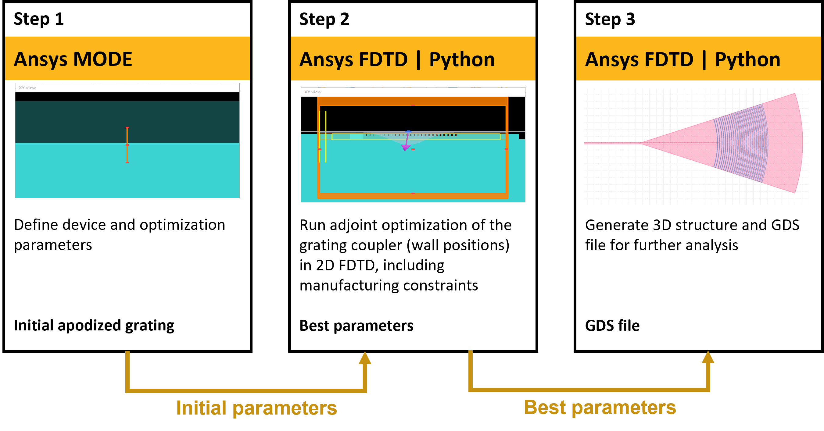
Lumerical's inverse design capability provides unparalleled optimization performance by combining the power of gradient-based optimization routine with efficiencies found in fundamental properties of Maxwell equations. This example will demonstrate how to use the inverse design method to generate a TE silicon on insulator (SOI) grating coupler design with maximized coupling efficiency. Moreover, we'll demonstrate how to modify the example with your parameters so you can reuse this approach for your own design.
This example draws extensively from the LumOpt framework:
- Photonic Inverse Design Overview - Python API
- Getting Started with lumopt - python API
- Optimizable Geometry - Python API
Step 1: Define base simulation in MODE
The goal for this initial step is to find a good starting point for the optimization. Using MODE FDE solver, we determine the initial linearly apodized grating based on the optimization parameters (central wavelength, etch depth, fiber angle).
Step 2: Optimization of the linearly apodized grating using 2D FDTD
The second step is to optimize the grating using a limited set of parameters. We use the apodized grating defined in step 1 as a starting point. The number of gratings is fixed at 25 and the etched depth at 80nm. A set of 4 parameters obtained from step 1, defining the grating apodization function, is used to extract the initial set of parameters to maximize transmission/coupling.
From the initial condition found in the previous step, we now run an optimization using the x coordinate of each wall position of the grating as a free parameter (2x 25 parameters).
Include manufacturing constraints
We run the 2D optimization enabling the minimum feature size constraint (set to 100nm) to make sure the device will be manufacturable.
Step 3: Extract 3D design and GDS file
The optimized grating coupler component shape with curved gratings will be exported into GDS II format and into a 3D simulation file which can be used for further simulation and/or fabrication (mask design). We used circular gratings that cover the source area to make sure that all the fiber light is collected. We also used a short linear taper to connect to a 450nm wide waveguide. The geometry of the gratings and taper can be further optimized by the designer.
Photonic Inverse Design: Grating Coupler (3D)
Run and results
Instructions for running the model and discussion of key results
Step 1: Define base simulation parameters
This step is not necessary if you want to run the example as is, however, it is required for modification of the base simulation file based on your needs.
- Open the simulation file pid_grating_coupler_preliminary_design.lms in MODE
- Modify the desired base simulation parameters, save the file.
- Open the script file pid_grating_coupler_preliminary_design.lsf
- Modify the parameters and run the script
For a given center wavelength λc
and a given etch depth e
, we can follow ref. [1] to design an optimized apodized grating based on physical arguments. Here, we only briefly sketch the derivation, for more details and precise definitions of the variables, see the reference.
The main idea is to use the local effective index of an apodized grating. Specifically, for each unit cell, the effective index is approximated using a linear interpolation as:
neff=Fn0+(1−F)nE
Where F
is the filling fraction, nO and nE
denote the effective indices of a mode propagating in a waveguide with the full height and the height of the partially etched structure, respectively.
To determine those effective indices, we use the MODE FDE solver. The calculation is performed for a silicon waveguide with height h=220nm
, using a refractive index of 3.47668 for silicon, and 1.44401
for the background material (SiO2).
We can write the Bragg condition for a grating with periodicity Λ
as
Λ=λcneff−nbgsinθ
Where θ
is the angle of the incoming beam.
For a linearly apodized grating, the filling factor varies with the position along the waveguide
F(x)=F0−R⋅x
R
is the apodization factor and F0
the initial filling fraction. In the ideal case, it should be 1 as we start with a solid waveguide, but we will use F0=0.95 to avoid extremely small trenches.
Using the linear apodization in the interpolated effective index:
neff(x)=F(x)n0+(1−F(x))nE=nE+F(x)Δn
We get the spatially varying period of the grating:
Λ(x)=λc(nE−nbgsinθ)+F(x)Δn
To find a good initial condition, we discretize the filling fraction Fi
and the pitch Λi
for each period.
So far, we only have 1 unknown, the factor R
. For a slightly more efficient optimization, we can include 4 optimization parameters:
p=[x0,R,a,b]
With
Fi=F0−R(xi−1−x0)
Λi=λca+Fib
And
a=nE−nbgsinθ
b=Δn
Note x0
and R are to be defined separately. We will set x0 to –2.5μm and we will use R=0.03μm−1
(see ref. [1]). If you change the materials, geometries, or polarization, you should perform sweeps of these values to find a suitable initial point (grating).
The script pid_grating_coupler_preliminary_grating_design.lsf will calculate the initial parameters and save them in the pid_grating_coupler_initial_params.json file to be used in the next step.
Step 2: Optimization of the linearly apodized grating using 2D FDTD
We first need to find the optimum position for the fiber.
- Open the python script file pid_grating_coupler_sweep_2D.py in FDTD script editor
- If needed, modify the parameters
- Run the script
This script will load the initial design from step 1 and run a parameter sweep fiber to determine the fiber position for optimal coupling.

The optimum position is found at 4.2μm
, with a transmission over 60%.
- Open the python script pid_grating_coupler_2D_apodized.py from FDTD script editor
- If needed, update the parameters, then run the script
- Open the script pid_grating_coupler_2D_1etch.py
- Run the script
In this step, we will use the parameters obtained from 1 to 3 and then extract the x coordinate of each wall position as free parameters. More specifically, the parameters will be the starting position of the grating, the width of the etch, and the width of the tooth of each grating.
The script pid_grating_coupler_2D_apodized.py will save to the file pid_optim_1.json these parameters, which can be used as a starting point.
We use the minimum feature size constraint in this step by setting min_feature_size=0.1, which will ensure that no trench is less than 100nm wide.
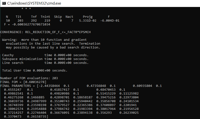
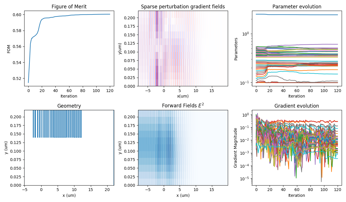
The final transmission is around 60% and now the grating coupler will be easily manufacturable. The optimized grating parameters are saved in pid_optim_final.json .
Step 3: Extract 3D design and GDS
- Open the script pid_grating_coupler_3D.py
- If needed, modify the settings
- Run the script
This script will load the results of the optimization, set the corresponding 3D simulation, and extract the GDS from the structure.
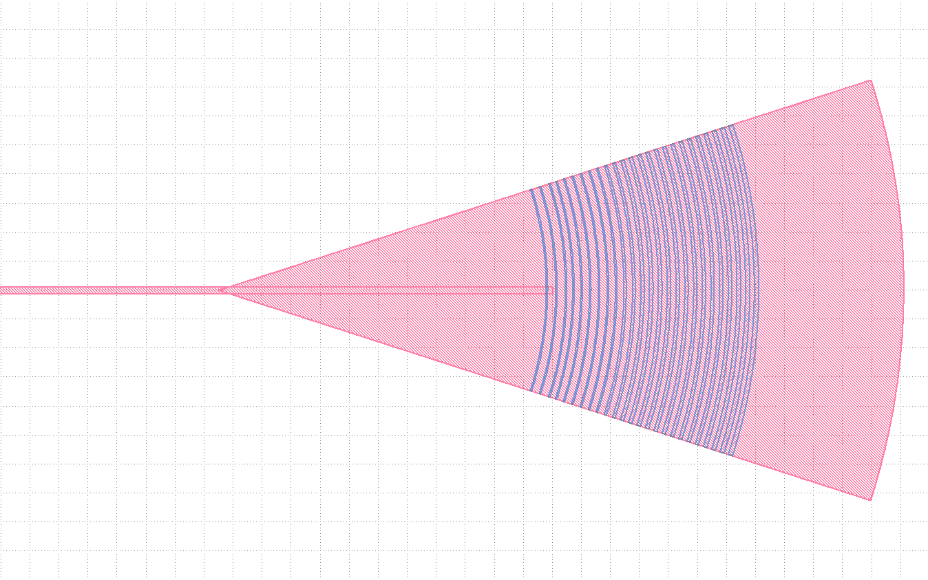
The 3D simulation can be used for further analysis and/or optimization. Note we should first determine the optimum fiber position with this 3D structure. The simulation file already includes a parameter sweep for that purpose.
| Note: Running the 3D simulations will require much more resources than the 2D ones. |
Important model settings
Description of important objects and settings used in this model
The main parameters of the optimization are set at the beginning of the scripts, and in the base simulation file pid_grating_coupler_2D_TE_base.fsp .
# Optimization global parameters
lambda_c = 1.55e-6
bandwidth_in_nm = 0 #< Only optimize for center frequency of 1550nm
F0 = 0.95
height = 220e-9
etch_depth = 80e-9
y0 = 0
x_begin = -5.1e-6
x_end = 22e-6
n_grates = 25

indexSi = 3.47668
indexSiO2 = 1.44401
Polarization : The chosen refractive index values are representative of an SOI chip manufacturing process. Because of the high refractive index contrast between silicon and silicon oxide, there is a large difference between effective indices of the two fundamental modes – TE and TM – of the integrated waveguide. For this reason, SOI grating couplers are strongly polarization selective. The presented design excites a TE mode since this is the most common choice, however, it is also possible to set up an optimization targeting the TM mode. To change the polarization to TM, or higher order mode, one needs to change the mode number in pid_grating_coupler_preliminary_design.lsf and in the ModeMatch class of the pid_grating_coupler python files. Also one should change the polarization angle in base fsp files. For TM optimization the mode number is 2 and the polarization angle is 0 degrees in this configuration.
Tilting angle : The coupling efficiency depends heavily on how the fiber meets the top silicon oxide cladding layer. In this example, we use a Gaussian beam as an approximation of the output of the beam from the fiber. The end of the fiber is assumed to be polished at a small angle so that the fiber tilts as it is mounted on the top cladding. Such tilting prevents reflections into the fiber.
Etch depth : The coupling efficiency is highly sensitive to the grating’s pitch, duty cycle, and etch depth. For simplicity, a fixed etch depth is employed here, however, it can also be varied if the available fabrication process provides that degree of freedom.
Substrate : If a silicon substrate is present in the fabricated device, it should be included in the simulations. The substrate will have a noticeable impact on how light is coupled and cannot be omitted as is often done in other device designs.
Optimization figure of merit (FOM) : The purpose of the design is to have the best possible coupling at a desired wavelength, the optimization figure of merit is chosen to be the transmission through the grating coupler at 1550nm, and the optimization algorithm will try to maximize this value. Lumopt uses mode power coupling, and when sweeping the source position we use the power transmission.
Definition of optimizable geometry : The optimizable geometry is defined as a polygon that has fixed values for the y coordinates of its boundary points and the points’ x coordinates can be modified to obtain the optimal geometry.
Optimization fields monitor : The optimization fields DFT monitor (opt_field) is used to collect the field data within the optimizable geometry which is then used to calculate field gradients used in the optimization algorithm. As such, the location of this monitor is of great importance and should cover the entire optimizable geometry.
Figure of merit fields monitor : Since this monitor is used to calculate the figure of merit required for optimization (mode overlap to the fundamental TE mode of the output waveguide), it should be located within the output waveguide of the grating coupler with appropriate dimensions.
Height of the geometry objects : The height (depth) of the geometry objects is chosen based on the fabrication/foundry process. This is especially important for the 3D simulation to ensure correct geometry setup. This is done by adjusting the “height” and “etch_depth” in the scripts. These values are also used in the script exporting the structure to a GDS file.
Optimization parameters bounds and initial values : The range over which the optimization algorithm is allowed to vary the parameters and also the initial values for those parameters as a starting point are defined by initial_params and bounds arrays as input arguments when calling the function FunctionDefinedPolygonI.
Optimization spectral range : The spectral range of the optimization can be specified as the array “wavelengths” as well as the number of frequency points considered in optimization. Note that choosing a large number of frequency points will make the optimization much slower and can cause issues when transferring a large amount of data between FDTD and the Python environment. It is recommended to keep this number as low as possible especially for 3D simulations. For a single frequency optimization, simply choose the same start and stop values with points set to 1.
Maximum number of iterations : While the algorithm has the capability to stop the optimization once the gradient of the figure of merit falls below a certain threshold, the “max_iter” variable used for defining the optimization algorithm can be used to limit the number of iterations the algorithm is able to perform.
Target FOM : The target values for FOM at different wavelengths can be specified with the "target_T_fwd" input argument when defining the FOM. This should be an array with the same length as wavelength data and contain target FOM values (forward transmission) for each wavelength which can be less than 1. The default is 1 for all wavelengths. This gives users the option to aim for a desired value of transmission within the design spectral range.
Updating the model with your parameters
Instructions for updating the model based on your device parameters
Geometry : If you need to have your own geometry defined for the grating coupler, including SOI device layer thickness (grating height) and etch depth, corresponding changes should be made in the base simulation file and/or optimization setup Python script. This might need changes in object span and location in the base script, the polygon’s “etch_depth” parameter in python script which its value is also passed to the GDS export portion of the script. The source, simulation region, mesh override, and field gradient and FOM monitors dimensions should also be adjusted accordingly to make sure they cover the entire structure properly.
In this example, we use the function FunctionDefinedPolygon to set the grating coupler geometry as a polygon. Alternatively, we can use ParametrizedGeometry instead, giving more flexibility in how the geometry is set. The scripts offer the possibility to switch from one to the other by commenting/uncommenting the corresponding lines in the function runGratingOptimization :
def runGratingOptimization(bandwidth_in_nm, etch_depth, n_grates, params, working_dir):

bounds = [(-4,3), #< Starting position (in um)
 (0,0.05), #< Scaling parameter R
 (1.5,3), #< Parameter a
 (0,2)] #< Parameter b

 # geometry = ParameterizedGeometry(func = etched_grating,
 # initial_params = params,
 # bounds = bounds,
 # dx = 1e-5)

 geometry = FunctionDefinedPolygon(func = grating_params_pos,
 initial_params = params,
 bounds = bounds,
 z = 0.0,
 depth = 110e-9,
 eps_out = indexSiO2 ** 2,
 eps_in = indexSi ** 2,
 edge_precision = 5,
 dx = 1e-5)
Materials : The permittivity of the materials included in the simulation (the material making the optimizable geometry (core) and the material surrounding it (cladding)) for the desired simulation wavelength should be passed to the optimizer when defining the geometry by calling the function FunctionDefinedPolygon (here they are presented as refractive index (n) squared). The refractive index (not permittivity) of the waveguides (which is the same as the optimizable geometry) should also be defined in the base simulation setup script.
Grating geometry : We used circular shape gratings for 3D simulations and GDS export. One can use more sophisticated grating shapes similar to focusing grating couplers .
Taking the model further
Information and tips for users that want to further customize the model
Taper optimization : The 3-D coupler model uses a linear taper section to connect to the integrated waveguide at the start of the grating. The coupling efficiency can also be improved by optimizing the taper shape (see SOI taper design).
High efficiency grating couplers : Couplers with an efficiency higher than 90% over a large bandwidth have been designed with FDTD using more sophisticated gratings and a mixed 2-D/3-D optimization strategy (see references).
Additional resources
Additional documentation, examples, and training material
Related publications
- R. Marchetti, C. Lacava, A. Khokhar, X. Chen, I. Cristiani, D. J. Richardson, G. T. Reed, P. Petropoulos and P. Minzioni, “High-efficiency grating-couplers: demonstration of a new design strategy,” Scientific Reports 7, Article number: 16670, 2017. ( https://www.nature.com/articles/s41598-017-16505-z );
- Neil V. Sapra et.al, “Inverse design and demonstration of broadband grating couplers” IEEE Journal of Selected Topics in Quantum Electronics ( Volume: 25, Issue: 3, May-June 2019 )
- D. Taillaert, F. Van Laere, M. Ayre, W. Bogaerts, D. Van Thourhout, P. Bienstman and R. Baets, “Grating Couplers for Coupling between Optical Fibers and Nanophotonic Waveguides,” Japanese Journal of Applied Physics, vol. 45, no. 8a, pp. 6071-6077, 2006.
- T. Watanabe, M. Ayata, U. Koch, Y. Fedoryshyn and J. Leuthold, “Perpendicular Grating Coupler Based on a Blazed Antiback-Reflection Structure,” Journal of Lightwave Technology, vol. 35, no. 21, pp. 4663- 4669, 2017.
See also
- Photonic Inverse Design Overview - Python API
- Getting Started with lumopt - python API
- Optimizable Geometry - Python API
- Grating coupler
- Broadband grating coupler
- MATLAB-driven grating coupler optimization
- SOI taper design
- Spot size converter
- Python API
- S-parameter simulator (SPS)
- S-parameter matrix sweep feature
- S-parameter file formats
Related Ansys Innovation Courses
Appendix
Additional background information and theory
Parametric Optimization (Adjoint method)
In a typical device optimization, the goal is to minimize or maximize a figure of merit F(p)
that depends on a set of N design parameters p=(p1,...,pn). The figure of merit can be any quantity used to benchmark the device’s performance and the design parameters can be any quantity that alters the device’s response. To evaluate F(p) for a given set of values of p, a physics-based modeling tool - such as FDTD - is used to map values of p to values of F. The model usually contains a description of the device’s geometry, materials, and all relevant environmental conditions. In a parameterized shape optimization, the goal is to allow some parts of the device’s geometry to vary to minimize or maximize the figure of merit. For this purpose, a shape function f(p)
is typically defined to specify part of the device’s geometry; an example is shown in the following figure:
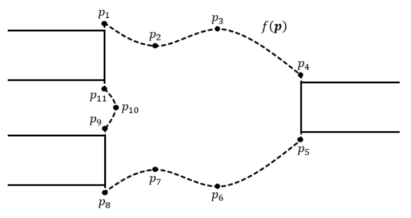
Y-splitter with a parameterized junction boundary f(p)
defined using connected splines.
The shape function is typically user-defined and must be fed to the modeling tool to construct the device’s geometry. Once the figure of merit F(f(p))
can be evaluated for a given shape function, a minimizer can make multiple evaluations of the figure of merit to find the optimal shape. There is a very large body of minimization tools and techniques that can be used to try to find the optimal shape parameters. When selecting a minimization technique, it is important to consider that running a device simulation to evaluate the figure of merit can be a slow operation. So, the best-suited minimization techniques are those that limit the number of evaluations of the figure of merit. With a good starting point, gradient-based methods can quickly find the optimal parameters with a relatively small number of figure of merit evaluations provided that it is also possible to evaluate the gradient of the figure of merit:
∇pF=(∂F∂p1,⋯,∂F∂pn)
To evaluate the gradient without having to perform one simulation for each partial derivative, a technique called the adjoint method can be employed. This technique exploits the properties of linear partial differential equations to evaluate the gradient using only two simulations independently of the number of optimization parameters. The Python-based shape optimization module in FDTD (lumopt) allows users to define a shape function and run the corresponding device simulation to evaluate the figure of merit. The module also implements the adjoint method to provide the gradient. In this way, any of the gradient-based minimizers in SciPy’s optimization module can be used to perform a fully automated optimization.
S-parameter extraction from component level simulations of passive photonic devices
The S-parameter matrix formalism is a common approach to build compact models of photonic devices to be used in circuit-level simulations . Assuming the response of the device to optical signals is linear, it can be modeled by a network (black box) with multiple network ports, where each of them receives an incoming signal and scatters or reflects an outgoing signal.
We assume the device has N physical ports (which typically are input/output waveguide channels) and each of these supports a certain number of modes of interest. Each element of the S-parameter matrix is the ratio between the complex envelopes of the optical modes in two physical ports. For example, to model the behavior of the fundamental TE and TM modes at the input/output waveguide channels of a 1x2 MMI we need a 6x6 S-parameter matrix, given that there are two modes at each of the three physical ports. Each column of the S-parameter matrix corresponds to a fixed input physical port and mode and each row corresponds to a fixed output physical port and mode.
The approach to extract the S-parameter matrix of a photonic device depends on the solver being used. In both FDTD and EME solvers, port objects can be set up at each of the physical ports. The main differences between the solvers for the S-parameter extraction are:
- FDTD injects one mode in one input port object per simulation, while EME can solve for all the elements of the S-matrix in one simulation;
- FDTD is broadband so many frequency points can be calculated in one simulation, while results from EME are for a single frequency per simulation.
Therefore, in both solvers, it is necessary to run sweeps to obtain the full S-parameter matrix at multiple frequency values, either by sweeping over the input physical ports and modes or over the frequency points.
Use the examples in the Application Gallery to determine the appropriate solver for your component. This section describes the recommended approach for S-parameter extraction and export to INTERCONNECT once you have determined the appropriate solver.
In this section we describe how to:
- For FDTD, calculate the S-parameter matrix and save it to a file with the appropriate format to be imported in an Optical N-port S-parameter primitive element in INTERCONNECT.
- For EME, calculate the S-parameter matrix and save it to a file with the appropriate format to be imported in an Optical N-port S-parameter primitive element in INTERCONNECT.
- Optionally, more accurately account for group delay of the device. This is important in elements that will be part of phase-sensitive circuits (for example, cavities, resonating structures, and interferometric devices). We will use the group delay specification in the S-parameter file , required for the group delay option in the digital filter of the Optical N-port S-parameter element in INTERCONNECT.
How to extract S-parameters (FDTD)
- Check that the port objects in the simulation have been set up correctly to collect all the data required for the S-parameter matrix. In particular, make sure that all the desired modes are selected at the ports; the “user select” option in the Modal Properties allows you to pick multiple modes (for example, fundamental TE and TM modes) when necessary for the full S-parameter matrix.
- Create an S-parameter matrix sweep item in the “Optimizations and Sweeps” window with the following settings:
- S-Matrix Setup tab:
- The modes selected at each port are displayed in this tab. Make sure the list is consistent with the physical ports and modes you want to include in the S-parameter matrix (see step 1).
- The option “Excite all ports” is enabled by default, which means that a simulation will be run for every port and mode in the list to calculate each column of the S-parameter matrix. To reduce the number of simulations you can map between columns taking advantage of symmetries in the structure. If that is the case, disable the “Excite all ports” option and click on the “Auto symmetry” button to let the solver determine the appropriate mapping based on the port locations. In some cases, adjustments to the mapping are required so it is always recommended to review the settings after applying auto symmetry.
- INTERCONNECT Export Setup tab:
- Select the “Custom define” option to define the mode ID and port location properties.
- The file export automatically assigns a mode ID to each mode. It is often necessary to manually set the mode ID so they are consistent with the orthogonal identifier convention to be used in INTERCONNECT. This is important, for example, when connecting the Optical N-port S-parameter element to an Optical Network Analyzer (ONA) in INTERCONNECT. The setting for the excitation mode in the ONA is the “orthogonal identifier” property in the “Waveguide” section. The typical convention is to use “orthogonal identifier” = 1 for the fundamental TE mode and “orthogonal identifier” = 2 for the fundamental TM mode.
- S-Matrix Setup tab:
- After running the S-parameter sweep, the “Visualize” and “Export to INTERCONNECT” options become available in the context menu of the S-parameter sweep item. The “Export to INTERCONNECT” option allows you to generate a text file with the S-parameters. This file has the format required by the Optical N-port S-parameter primitive in INTERCONNECT without group delay specification, which is appropriate when the phase or group delay of the device are not critical for the compact model.
- If phase and group delays are critical, the group delay can be estimated by calculating the slope of the phase as a function of frequency at the center frequency/wavelength. The script add_group_delay_FDTD_Spar.lsf takes as input the S-parameter text file created in step 3 and modifies it to include the group delay. For more information see the section S-parameter extraction for group delay option in INTERCONNECT below.
How to extract S-parameters (EME)
- Create a parameter sweep in the “Optimizations and Sweeps” window with “model::EME::wavelength” as a parameter and “::model::EME::user s matrix” as a result; this sweep will run multiple simulations with different wavelengths. An alternative is to use the “Wavelength sweep” feature in the EME Analysis window , which will use only one simulation to quickly estimate the S-parameters over a given wavelength range; however, this feature should not be used to obtain final results as the accuracy of the calculation depends on the type of simulated structure.
- Examples that use EME include a script that exports S-parameters in the format required by the Optical N-port S-parameter primitive. In the script, you need to provide the INTERCONNECT port definitions (names and locations) and the S-parameter file name. The following actions are performed by the script:
- Run the parameter sweep for wavelength, collect the results and write them in the text file with the appropriate format.
- In situations where the phase and group delay are critical, the script will also run the simulation and the EME propagation for the center wavelength with the option “calculate group delays” enabled. The group delay is added to the text file and the S-parameter phase is corrected as explained below in the section S-parameter extraction for group delay option in INTERCONNECT .
- The output of the script is the S-parameter text file in the correct format ready to be imported in INTERCONNECT.
S-parameter extraction for group delay option in INTERCONNECT
Some photonic circuits rely on controlling the phase of the optical signal traveling through the different components; therefore, the phase of the S-parameters can be very important. There are a couple of challenges to capture the phase correctly in the Optical N-port S-parameter primitive in INTERCONNECT:
- A spectral sampling of the phase in the S-parameter data: Typically, the variation of the phase as a function of frequency is mostly linear with a slope that is proportional to the group delay (the delay of the optical signal between two ports). Therefore, in long devices, the phase can change very quickly with frequency, and a fine sampling in frequency would be necessary to avoid phase changes greater than 2π
- so that the phase has the correct slope after unwrapping it. This is important for both frequency- and time-domain simulations in INTERCONNECT.
- Capturing the correct group delay and frequency dependence of the S-parameters in INTERCONNECT time-domain simulations: For time-domain simulations, the most common type of filter used in the Optical N-port S-parameter primitive is the finite impulse response (FIR) one, which has multiple options for the estimation of taps. The choice depends on what is the most significant aspect of the element response to be captured in the circuit simulations. In elements where the phase is important, typically it is necessary to capture both the group delay and the frequency dependence of the S-parameters correctly.
The “group delay” option for the “number of taps estimation” in the digital filter settings of the Optical N-port S-parameter primitive provides solutions to both challenges:
- The group delay is captured correctly without requiring a fine spectral sampling of the S-parameters by using group delay estimates provided by the user for each S-parameter matrix element at the center frequency/wavelength.
- In most cases, the FIR filter in time-domain simulations can capture the group delay and frequency dependence of the element response more accurately with the "group delay" option, compared to other options for tap estimation. With the "group delay" option, the number of taps available to the filter depends on the sample rate of the INTERCONNECT simulation and the group delay estimate provided by the user: for a given sample rate, there are more taps available for larger group delays. Since most photonic devices are long compared to the wavelength of the signal, typically the number of available taps is not a concern. Only in cases where the device is relatively short, it might be necessary to increase the sample rate.
Compared to the regular file format for S-parameter files in INTERCONNECT, the group delay option requires a slightly different format , which includes the group delay estimate in the header of each S-parameter data block; furthermore, the phase provided in the file needs to be adjusted to remove the linear contribution associated with the group delay estimate. The previous section describes how this type of file can be generated when using FDTD or EME for the S-parameter extraction. For more information on the group delay option see the discussion here .
INTERCONNECT application example
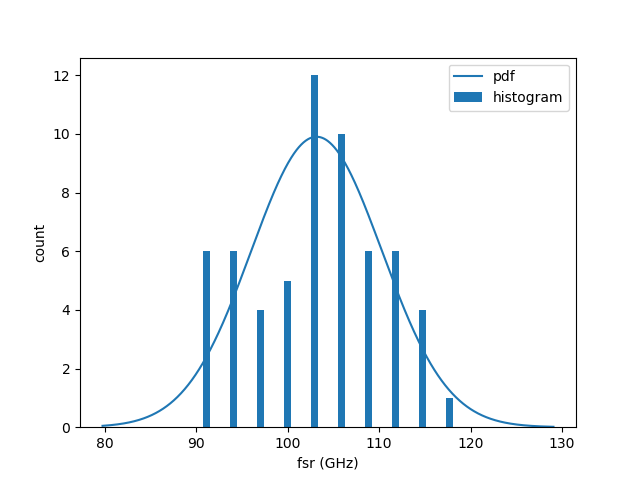
This example demonstrates the feasibility of integrating Lumerical INTERCONNECT with Python. This interoperability is made possible using Application Programming Interface (API). In this example, a Monte Carlo analysis in INTERCONNECT will be generated using Python script based on the circuit defined in the file run_monte_carlo.icp and some of the results such as the histogram and probability density function (pdf) will be plotted using Python plot functions.
This example is similar to the Monte Carlo scripting commands example in the Parameter sweeps, Optimization and Monte Carlo analysis section.
Requirements: Lumerical products 2018a R4 or newer
| Note:
|
During the Lumerical product installation process, a lumapi.py file should be automatically installed in this location.
| Linux | /opt/lumerical/interconnect/api/python/ |
| Windows | C:\Program Files\Lumerical\<version>\interconnect\api\python |
This module is the key to enable Lumerical-Python API connection. Once the lumapi module is imported to Python, the integration should be ready. See this page for instructions for setting up Python API.
Importing modules
The following script lines imports the modules ( imp and matplotlib ) and the Lumerical Python API that will be used in the later script.
import importlib.util
#The default paths for windows, linux and mac
spec_win = importlib.util.spec_from_file_location('lumapi', 'C:\\Program Files\\Lumerical\\2020a\\api\\python\\lumapi.py')
spec_lin = importlib.util.spec_from_file_location('lumapi', "/opt/lumerical/2020a/api/python/lumapi.py")
spec_mac = importlib.util.spec_from_file_location('luampi', "/Applications/Lumerical/FDTD Solutions/FDTD Solutions.app/Contents/API/Python/lumapi.py")
#Functions that perform the actual loading
lumapi = importlib.util.module_from_spec(spec_win) #
spec.loader.exec_module(lumapi)

from matplotlib import pyplot as pyplot
User can also use the method mentioned in the Session management - Python API
Creating the Monte Carlo analysis
The following line loads and opens the INTERCONNECT project file run_monte_carlo.icp . An INTERCONNECT instance will be opened up by this.
ic = lumapi.INTERCONNECT("run_monte_carlo.icp")
The following commands generate and superficially define a new Monte Carlo analysis named "MC_script". The use of dictionary data type in Python separates the setup data from the function calls to setsweep , and makes the code cleaner to manage.
ic.addsweep(2)
MC_name = "MC_script"
ic.setsweep("Monte Carlo analysis", "name", MC_name)

setup = {
    "number of trials": 200.0,
    "enable seed": 1.0,
    "seed": 1.0,
    "Variation": "Both",
    "type": "Parameters",
}

for k, v in setup.items():
    ic.setsweep(MC_name, k, v)
After the Monte Carlo analysis object is superficially generated, the parameters can then be defined and added to it. Each of the parameters is defined as a Python dictionary (they are structs inside Lumerical script), and we use an array to store these parameter dictionaries to later loop over to add to the Monte Carlo analysis object.
sweep_parameters = [
    {
        "Name": "cpl_2",
        "Parameter": "::Root Element::WC2::coupling coefficient 1",
        "Value": ic.getnamed("WC2", "coupling coefficient 1"),
        "Distribution": {
            "type": "gaussian",
            "variation": 0.02
        }
    },
    {
        "Name": "cpl_3",
        "Parameter": "::Root Element::WC3::coupling coefficient 1",
        "Value": ic.getnamed("WC3", "coupling coefficient 1"),
        "Distribution": {
            "type": "uniform",
            "variation": 0.04
        }
    },
    {
        "Name": "wgd_model",
        "Model": "WGD::group index 1",
        "Value": ic.getnamed("SW1", "group index 1"),
        "Process": {
            "type": "uniform",
            "variation": 1.02
        },
        "Mismatch": {
            "type": "gaussian",
            "variation": 0.1
        }
    },
    {
        "Name": "wgd_corr",
        "Parameters": "SW1_group_index_1,SW2_group_index_1,SW3_group_index_1",
        "Value": 0.95
    }
]

for parameter in sweep_parameters:
    ic.addsweepparameter(MC_name, parameter)
The next step is to add the results (free spectral range, bandwidth and gain) to this Monte Carlo analysis. The commands below add the results to the Monte Carlo analysis object and the results are defined in the array sweep_results . Again, each of the results is defined as a Python dictionary.
sweep_results = [
    {        "Name": "fsr",
        "Result": "::Root Element::Optical Network Analyzer::input 2/mode 1/peak/free spectral range",
        "Estimation": True,
        "Min": 1.0e11,
        "Max": 2.0e11
    },
   {        "Name": "bd",
        "Result": "::Root Element::Optical Network Analyzer::input 1/mode 1/peak/bandwidth",
        "Estimation": False
    },
    {        "Name": "gain",
        "Result": "::Root Element::Optical Network Analyzer::input 1/mode 1/peak/gain",
        "Estimation": False
    }
]

for result in sweep_results:
    ic.addsweepresult(MC_name, result)
The Monte Carlo analysis tab will look like below after the definition of the parameters and results:
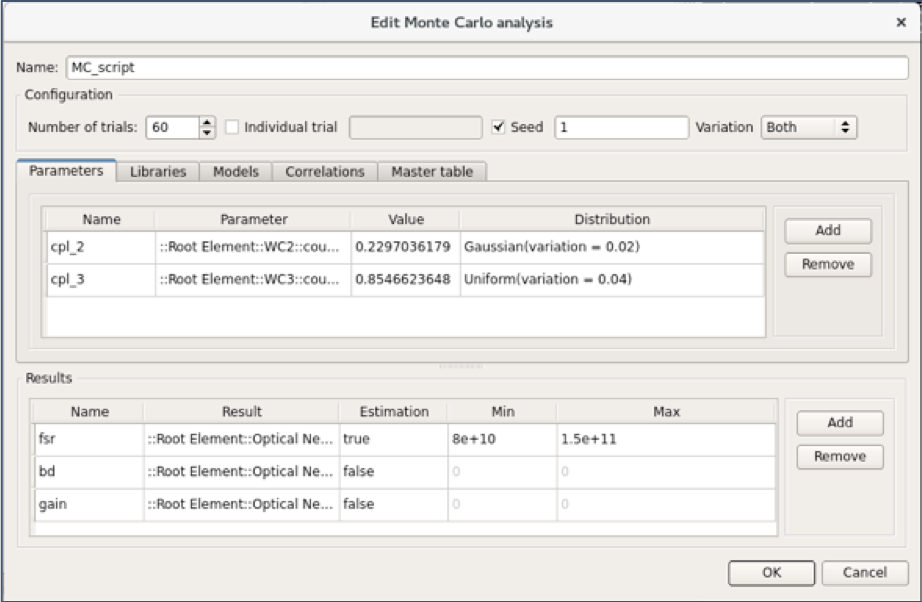
Running the Monte Carlo analysis
The following command runs the Monte Carlo analysis that defined in the previous step. The Monte Carlo analysis runs 60 trials in batches of 10 or less and automatically updates the analysis status window after each batch of trials.
ic.runsweep(MC_name)
Plotting the results
One of the advantages of using the Lumerical Python API is that we can take advantage of the advanced Python modules. In this example, we use pyplot in the matplotlib module to plot the Monte Carlo analysis results.
The following commands plot the FSR histogram and the estimation of its pdf in the same figure and this cannot be achieved by using Lumerical script commands.
fsr = ic.getsweepresult(MC_name, "analysis/results/histogram/fsr")
fsrCount = fsr["count"][0][0]
fsr = fsr["fsr"][0][0]

pdf = ic.getsweepresult(MC_name, "analysis/results/pdf/fsr")
pdfCount = pdf["count"][0][0]
pdfFsr = pdf["fsr"][0][0]

pyplot.bar(fsr/1e9, fsrCount)
pyplot.plot(pdfFsr/1e9, pdfCount)
pyplot.xlabel("fsr (GHz)")
pyplot.ylabel("count")
pyplot.show()
The plot is shown below:

Python co-simulation with INTERCONNECT

In this example, we show how an INTERCONNECT time domain simulation can be driven from Python using Lumerical’s Python API. We provide example scripts that show how to use the cosimulation commands runitialize , runstep , setvalue , getvalue and runfinalize to control an INTERCONNECT time domain simulation while setting and getting signal values at desired ports.
| Note:
|
Python co-simulation with INTERCONNECT
The problem we consider is a simple optical transceiver that can be operated in a variable speed mode. The setup consists of a CW laser (with RIN of -120 dB/Hz and power of 10 dBm) that feeds an ideal modulator. The light then passes through an attenuator and into a PIN photodiode (PD) where it is converted back to an electric signal. The PD includes a dark current of 0.1 mA and thermal noise of 1e-10 A/sqrt(Hz). The PD is followed by a low pass filter with a cutoff frequency of 10 GHz, to simulate the frequency response of the PD. The output is then forked. One fork is fed to a low pass filter with cutoff frequency of 0.2 GHz which can be used to monitor the optical power arriving at the PD. The second fork is fed to 2 eye diagram monitors – one measuring an eye at 25 GB/s and the other at 10 GB/s.
What is unusual about this setup is that the modulator is being driven by an EDA Cosimulation element . Furthermore, the Cosimulation element is also connected to the output of the monitoring signal, as well as the main output.
The co-simulation can be driven by Lumerical script and/or Python. The code will allow us to design control circuitry that switches the transceiver into operation at 25GB/s if the monitor power shows that the signal arriving on the detector is high enough. We can then look at the dynamics of the transition from 10GB/s operation to 25GB/s operation.
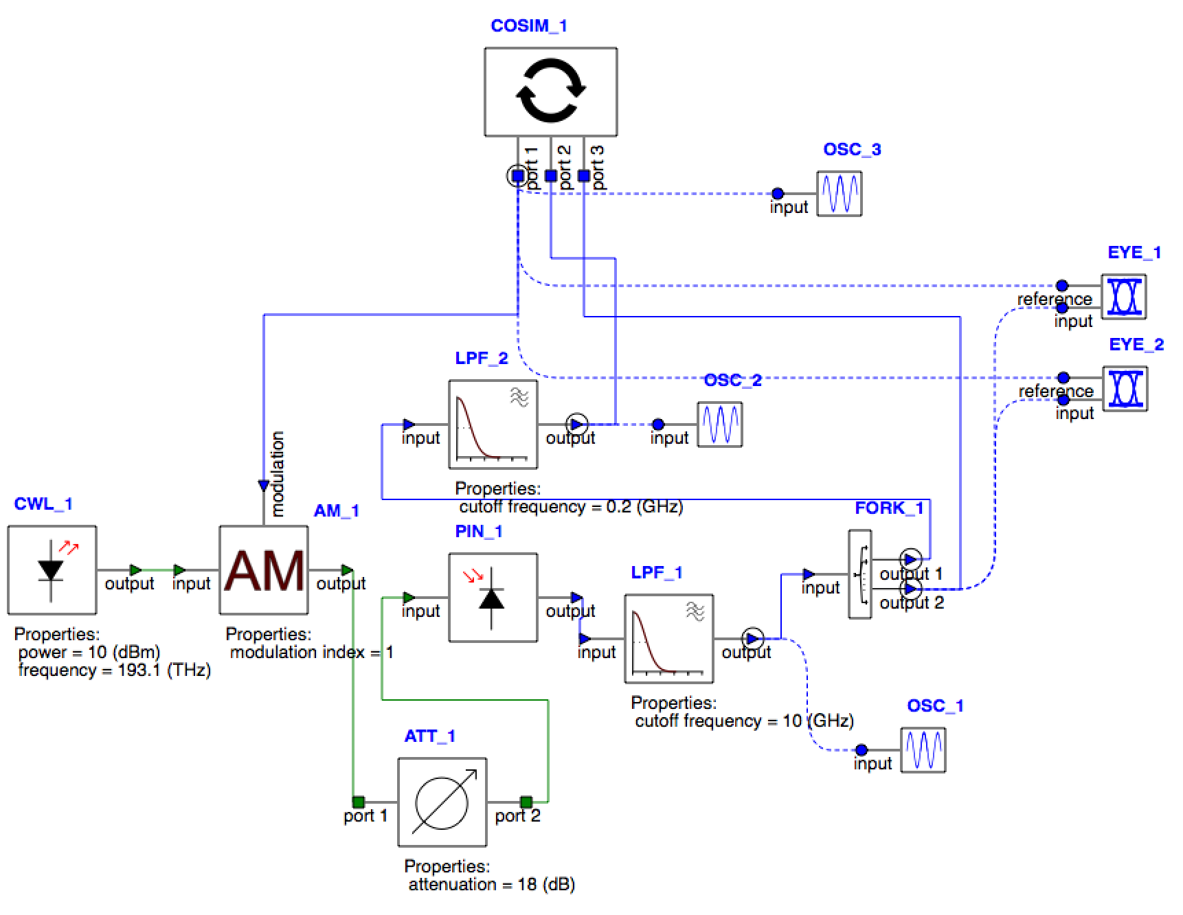
Simulation in Lumerical script
Simulation in Lumerical script
Open the .icp file co_simulation_example.icp with INTERCONNECT and the script file co_simulation_example.lsf . First, set the variable "target_speed" to “low” and run the script. Also, set the attenuator to 10 dB.
The script will plot the driving electrical signal, which is made up of an ideal NRZ signal of bits from a pseudo-random sequence, the signal used to monitor the optical power arriving at the PD and the output from the PD.
|
Signal driving the ideal modulator |
Monitoring signal |
Output from the PD |
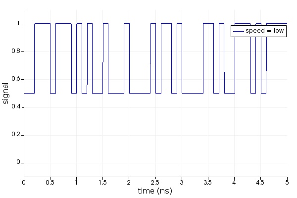
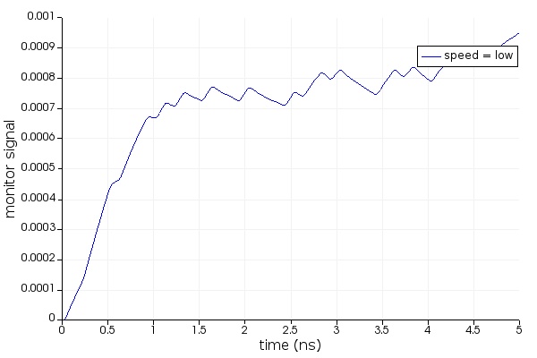
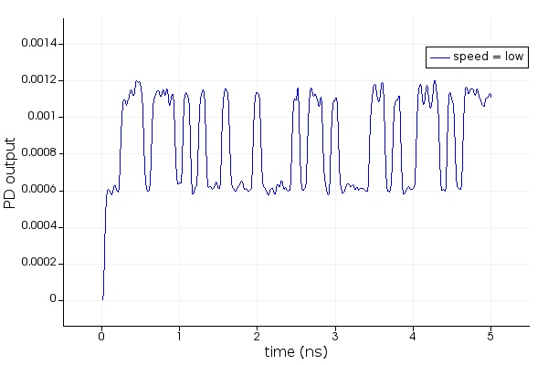
To visualize the eye diagram for the low speed co-simulation, you can go to "EYE_2" and right click and select "display results". The eye diagram is open well and the BER is estimated to be approximately 1e-19.
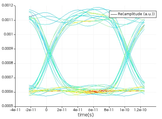
Next, change the "target_speed" variable to “high” and rerun the script. This will run the same transceiver at 25GB/s. The driving signal and output signal are shown below.
|
Signal driving the ideal modulator |
Output from the PD |
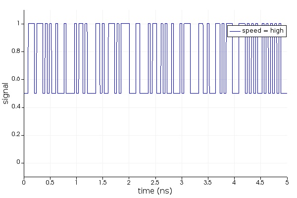
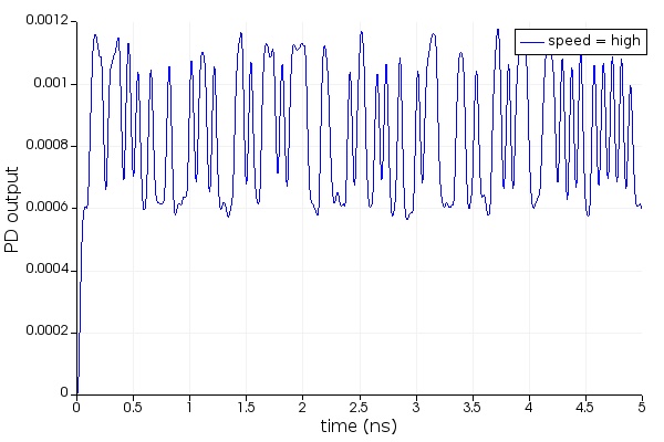
If we now display the results of the element "EYE_1", recording the eye at 25 GB/s, we see that it is still open, however, the BER is estimated to be about 2.5e-9.
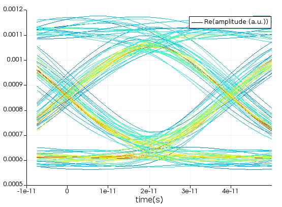
If we change the attenuator to have a loss of 18 dB, we can rerun and now see that the eye is closed.

After analysis of the previous results, we can set our "target_speed" to “variable” and our "conversion_threshold" to 0.0005. Once the monitor signal stays above the conversion threshold for at least the length of one bit, we switch from low speed to high speed.
If we switch the attenuator back to 10 dB, we see the following results.
|
Signal driving the ideal modulator |
Output from the PD |
|
Monitoring signal |
The operating speed switches from 10 GB/s to 25 GB/s |


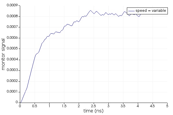
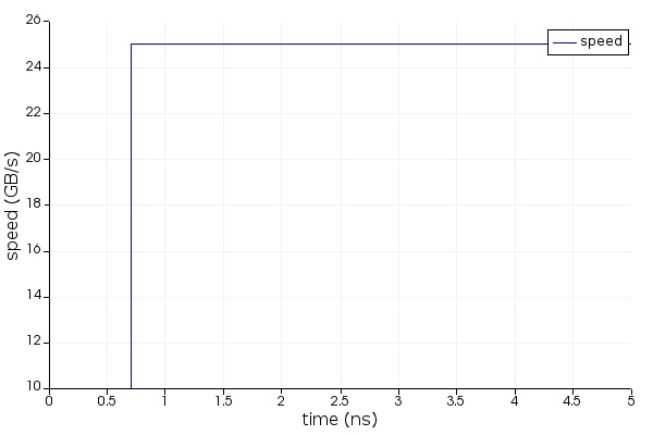
If we view the 25 GB/s eye diagram we can see that the eye is mostly open. The errors come from the early part of the signal where we were operating at only 10 GB/s, so this transition period would be lost communication time.
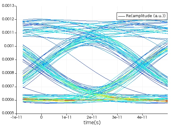
Simulation in Python
We can repeat everything in Python. To do this, the Python API must be configured and you must have a license. Please see Python API for more details.
For this example, we have used Lumerical script commands driven from Python to display results for easy comparison, but data visualization could be done directly in Python. At the end of the simulation, we pause the Python with pdb.set_trace(). This allows you to use the INTERCONNECT UI to display results before the window is closed. You can observe the simulation runs much more slowly with the Python API than from the Lumerical script, and this is something that Lumerical will be improving in the future.
|
Bit sequence from Lumerical script |
Bit sequence from Python |
|
Output signal from Lumerical script |
Output signal from Python |


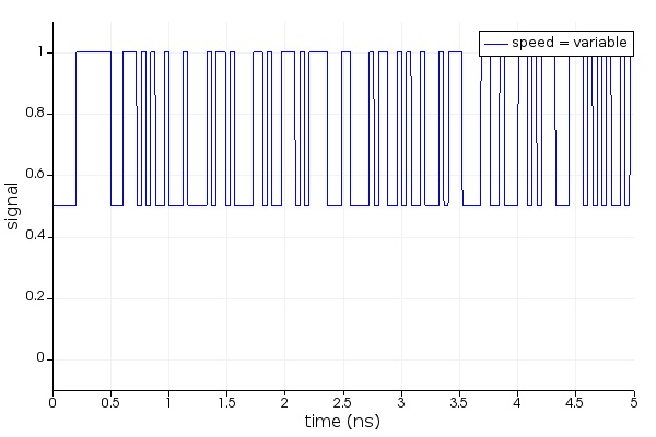
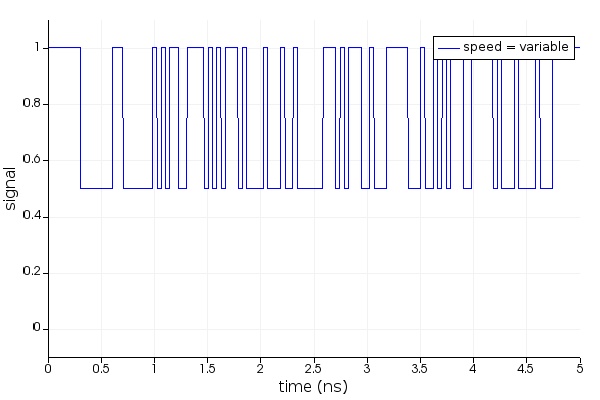
The differences between the bit sequences are because of a different random number generator. When the co-simulation pauses, we can go to the INTERCONNECT file to visualize the eye diagram. The eye diagram is offset due to the uncertainty in the transition time from 10 GB/s to 25 GB/s operation but it is clearly open.
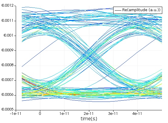


 1044
1044

 被折叠的 条评论
为什么被折叠?
被折叠的 条评论
为什么被折叠?
 到【灌水乐园】发言


