car::scatterplotmatrix散点图矩阵参数详解

最新推荐文章于 2022-10-06 09:31:53 发布

weixin_43230383

最新推荐文章于 2022-10-06 09:31:53 发布

阅读量3.4k

点赞数 7

分类专栏： R语言

原文链接：https://blog.csdn.net/qq_20828983/article/details/95659791

版权

R语言专栏收录该内容

7 篇文章 2 订阅

订阅专栏

转载自：https://blog.csdn.net/qq_20828983/article/details/95659791

在R语言实战第二版书，第八章回归分析时，用到了scatterplotmatrix 函数绘制散点图矩阵，发现已经不是当前最新的car包了，函数参数都错误了。在网上百度发现基本没有关于此函数的详细介绍，只有自己动手，查看help了。趁热打铁，写个说明。

基于的car版本为：3.0-3

附scatterplotMatrix函数源码：

先看函数的用法：

scatterplotMatrix(formula, data=NULL, subset, ...)
scatterplotMatrix(x, smooth = TRUE,
id = FALSE, legend = TRUE, regLine = TRUE,
ellipse = FALSE, var.labels = colnames(x), diagonal = TRUE,
plot.points = TRUE, groups = NULL, by.groups = TRUE,
use = c("complete.obs", "pairwise.complete.obs"), col =
carPalette()[-1], pch = 1:n.groups, cex = par("cex"),
cex.axis = par("cex.axis"), cex.labels = NULL,
cex.main = par("cex.main"), row1attop = TRUE, ...)
spm(x, ...)

下面对每个参数进行解释

scatterplotMatrix(x,
#smooth = list(spread = T, col.smooth = "black", col.spread = "black", lty.smooth=2, lwd.smooth=3, lty.spread=3, lwd.spread=2)
smooth = TRUE, #平滑曲线（多次拟合）False不绘制拟合曲线，True绘制，不分组则按全体，分组则按分组拟合。
#id 控制点标识；如果为false（默认），则不标识任何点；可以是 ShowLabels 函数的命名参数列表；
#true相当于list（method=“mahal”，n=2，cex=1，location=“lr”），
#它用最大的maha标识2个点（在每个组中，如果为by.groups=true）与数据中心的距离；
#不允许使用列表（method=“identify”）进行交互点标识。
id = FALSE,
#legend 图例默认legend = TRUE 为 legend = list(coords= "topright"),
#可以是一个列表，其中命名的elementcoords以图例函数可接受的任何形式指定图例的位置；
#c("bottomright", "bottom", "bottomleft", "left", "topleft", "top", "topright", "right", "center")
legend = TRUE, #根据分组绘制图例，并控制图例的位置；如果为false，则不绘制图例。
#regline 控制向每个绘图或每组点添加一条拟合回归线（如果by.groups=true）
#如果regline=false，则不绘制任何线条。
#此参数也可以是具有命名列表的列表，默认regline=true相当于regline=list（method=lm，lty=1，lwd=2，col=col[1]），
#指定计算行的函数的名称，行类型1（solid）的相对行宽为2，颜色等于a中的第一个值。
#设置method=MASS::rlm将使用稳健回归拟合。
regLine = TRUE, #回归线，TRUE绘制，flase不绘制
#ellipse 控制绘制数据集中椭圆。如果为“false”（默认），则不绘制椭圆
#可以是给定水平命名值的列表，或者一个向量的一个或多个二元正态概率等值线水平，在其中绘制椭圆；
#鲁棒性，确定是否使用质量包中的cov.trob函数来计算数据椭圆的中心和协方差矩阵的逻辑值。
#以及fill and fill.alpha，它控制椭圆是否被填充以及填充的透明度。
#true相当于list（levels=c（.5，.95），robust=true，fill=true，fill.alpha=0.2）
ellipse = FALSE,
var.labels = colnames(x), #变量标签（用于绘图的对角线）通过字符串可控制对角线标签位置
#diagonal 绘图对角线面板的内容。如果对角线=true，则绘制自适应核密度估计，
#如果存在分组，则分别为每个组绘制。对角线=false 取消对角线条目。可为：
#diagonal = list(method="adaptiveDensity", bw=bw.nrd0, adjust=1, kernel=dnorm, na.rm=TRUE) #核密度图
#diagonal=list(method="density", bw="nrd0", adjust=1, kernel="gaussian", na.rm=TRUE) #非自适应核密度估计
#diagonal=list(method ="histogram", breaks="FD") #直方图忽略分组
#diagonal=list(method="boxplot") #箱线图
#diagonal=list(method="qqplot") #normal QQ plot QQ图
#diagonal=list(method="oned") #倾斜于对角线的地毯图
diagonal = TRUE,
plot.points = TRUE, #如果为真，则在每个非对角面板中绘制点。
groups = NULL, #将数据分组的因子或其他变量；用不同的颜色和打印字符打印组。
by.groups = TRUE, #如果为真，则默认值、回归线和平滑将按组匹配。
#use 如果“complete.obs”（默认），则省略缺少数据的案例；
#如果“pairwise.complete.obs”），则在绘图的每个面板中使用所有有效案例。
use = c("complete.obs", "pairwise.complete.obs"),
#col 点的颜色；默认为从第二种颜色开始的轮盘。
#Regline和Smooth的颜色与第一组点的颜色相同，但可以在Regline和Smooth参数中进行更改。
col = carPalette()[-1], #col = c("red", "green3", "blue")
pch = 1:n.groups, #为点绘制形状；默认为按顺序绘制字符（请参见par）。 pch = c(15,16,17)
cex = par("cex"), #绘制点的相对大小
cex.axis = par("cex.axis"), #坐标轴标签的相对大小
cex.labels = NULL, #对角线上标签的相对大小
cex.main = par("cex.main"), #主标题的相对大小（如果有）
row1attop = TRUE, #如果为true（默认值），第一行位于顶部，false则颠倒。
...)

为了方便理解，这里使用基础包中的mtcars数据，边解说，边绘图。

一睹为快

先一睹为快，看最代码和图：

car::spm(~mpg + hp + wt, data = mtcars, groups = mtcars$gear, by.groups = F,
smooth=list(lty.smooth=2,lwd.smooth = 3, col.smooth="red", spread = T, lty.spread=3, lwd.spread=2),
diagonal = list(method="boxplot"), regLine=list(method =lm,lty=1,lwd=2,col="black"),
legend = list(coords= "topleft"),
var.labels = c("\n\n\nMPG\n(pg/ml)", "\n\n\nHP\n(μmol/L)", "\n\n\nWT\n(pg/ml)"),
cex = 1, cex.labels = 1.5, cex.axis = 1.5,
pch = c(16,16,16), col = c("red", "green3", "blue"), row1attop = T )

先加载程序包：

library(car)

1、数据添加

两种方式，1是用formula 格式指定数据框中的数据， 2是直接矩阵或者数据框：

car::scatterplotMatrix(mtcars[c("mpg", hp, wt)])
car::scatterplotMatrix(mtcars[c("mpg", "hp", "wt")])

结果如图：

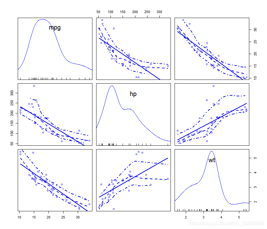
2、smooth 参数

平滑拟合曲线参数，False不绘制拟合曲线，True绘制，不分组则按全体拟合，分组则按分组拟合。

car::scatterplotMatrix(mtcars[c("mpg", "hp", "wt")], smooth = F)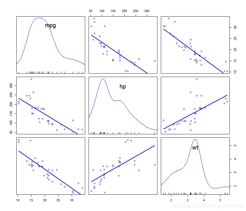

可以通过list修改拟合曲线参数。默认True时，拟合曲线参数为：

smooth=list(smoother=loessLine, spread=TRUE, lty.smooth=1, lwd.smooth=1.5, lty.spread=3, lwd.spread=1)

可以更改添加的线条的平滑度、线条类型、宽度和颜色以及添加平滑度参数等。

smoother表示拟合曲线方法，有：loessLine、gamline、quantregLine，各种方法的拟合曲线原理公式我是不知道了，各位看官如果知道，请给我说下。

Spread 表示是否绘制置信区间？？，我猜的，反正False时，两条边上的曲线没了。如图：

car::scatterplotMatrix(mtcars[c("mpg", "hp", "wt")], smooth = list(spread = F))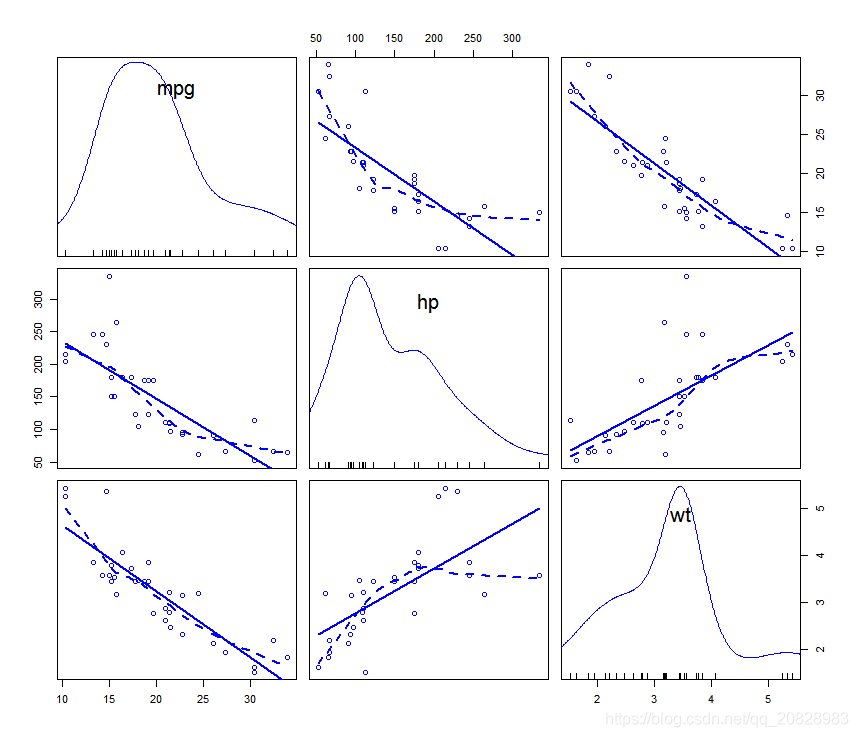

lty.smooth, lty.spread 修改曲线的线条类型， lwd.smooth和lwd.spread修改曲线的宽度

car::scatterplotMatrix(mtcars[c("mpg", "hp", "wt")],
smooth = list(spread = T, lty.smooth=2, lwd.smooth=3, lty.spread=3, lwd.spread=2))

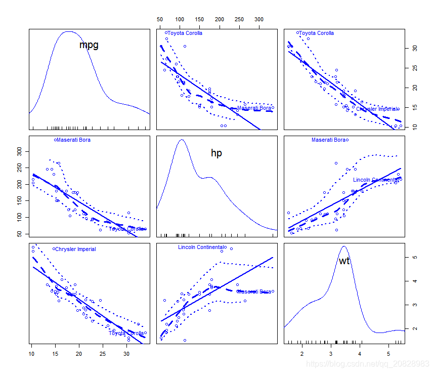
3、id 控制点标识

如果为false（默认），则不标识任何点；可以是 ShowLabels 函数的命名参数列表；true相当于，

id = list（method=“mahal”，n=2，cex=1，location=“lr”）

它用最大的maha标识2个点（在每个组中，如果为by.groups=true）与数据中心的距离；不允许使用列表（method=“identify”）进行交互点标识。这个我没改过，直接用默认True，标出离群点，如下图：

car::scatterplotMatrix(mtcars[c("mpg", "hp", "wt")], id = T,
smooth = list(spread = T, lty.smooth=2, lwd.smooth=3, lty.spread=3, lwd.spread=2))

后续很多参数需要用到分组，这里先把分组讲了

4、groups分组

和许多其他绘图函数一样，这里需要传入一个分组数据：groups = mtcars$gear

car::scatterplotMatrix(mtcars[c("mpg", "hp", "wt")],
smooth = list(spread = T, lty.smooth=2, lwd.smooth=3, lty.spread=3, lwd.spread=2),
id = T, groups = mtcars$gear )

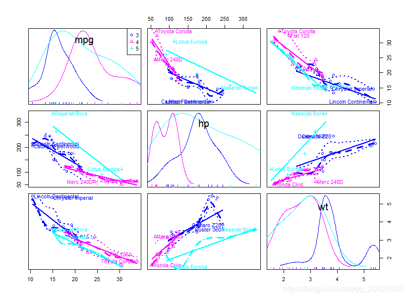
很多时候，我们不需要将每组进行拟合，而是想将整体数据进行拟合，这时我们需要修改参数：

by.groups = F，（Flase表示不需要每组进行拟合）

car::scatterplotMatrix(mtcars[c("mpg", "hp", "wt")],
smooth = list(spread = T, lty.smooth=2, lwd.smooth=3, lty.spread=3, lwd.spread=2),
id = T, groups = mtcars$gear, by.groups = F )

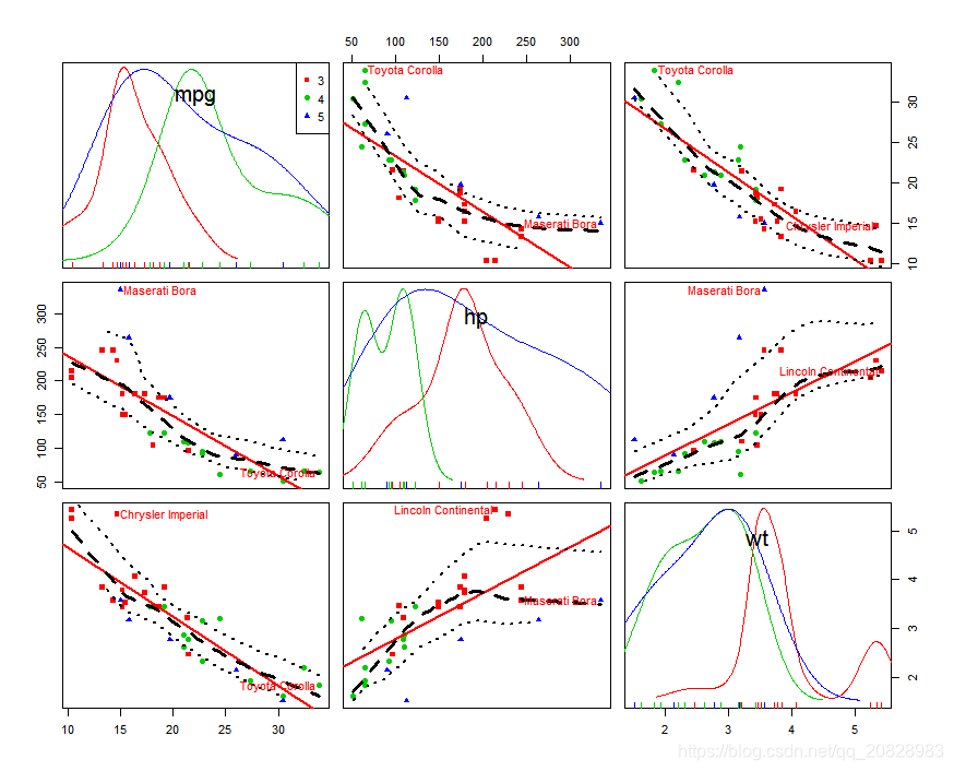
上面点的颜色和形状太难看了，需要修改下参数如下：

pch = c(15,16,17), #由于我们分了3组，所有这里只需要3个数据

col = c("red", "green3", "blue")

car::scatterplotMatrix(mtcars[c("mpg", "hp", "wt")],
smooth = list(spread = T, col.smooth = "black", col.spread = "black",
lty.smooth=2, lwd.smooth=3, lty.spread=3, lwd.spread=2),
id = T, groups = mtcars$gear, by.groups = F,
pch = c(15,16,17),col = c("red", "green3", "blue"))

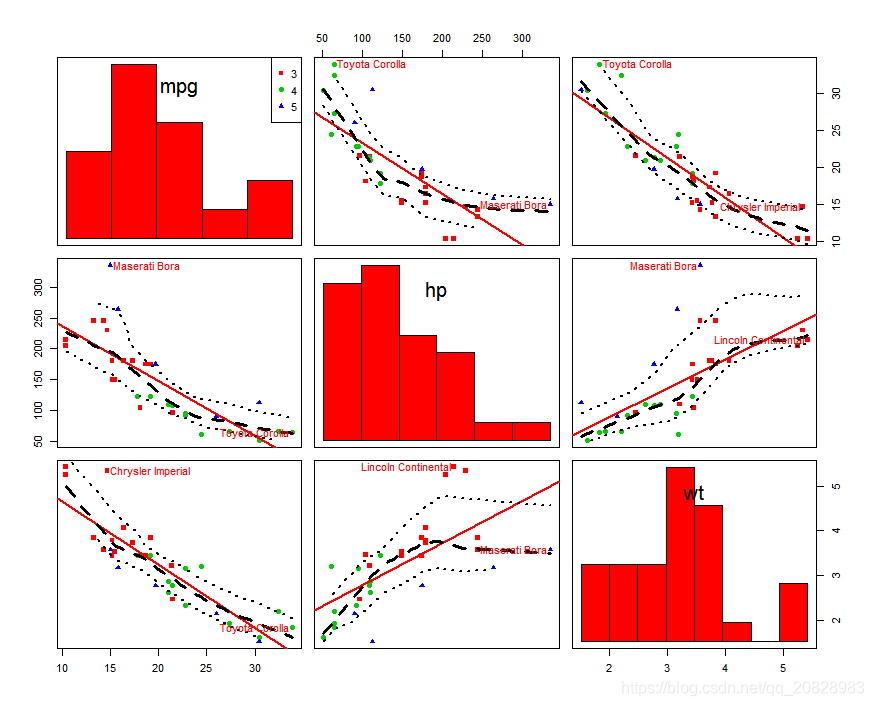
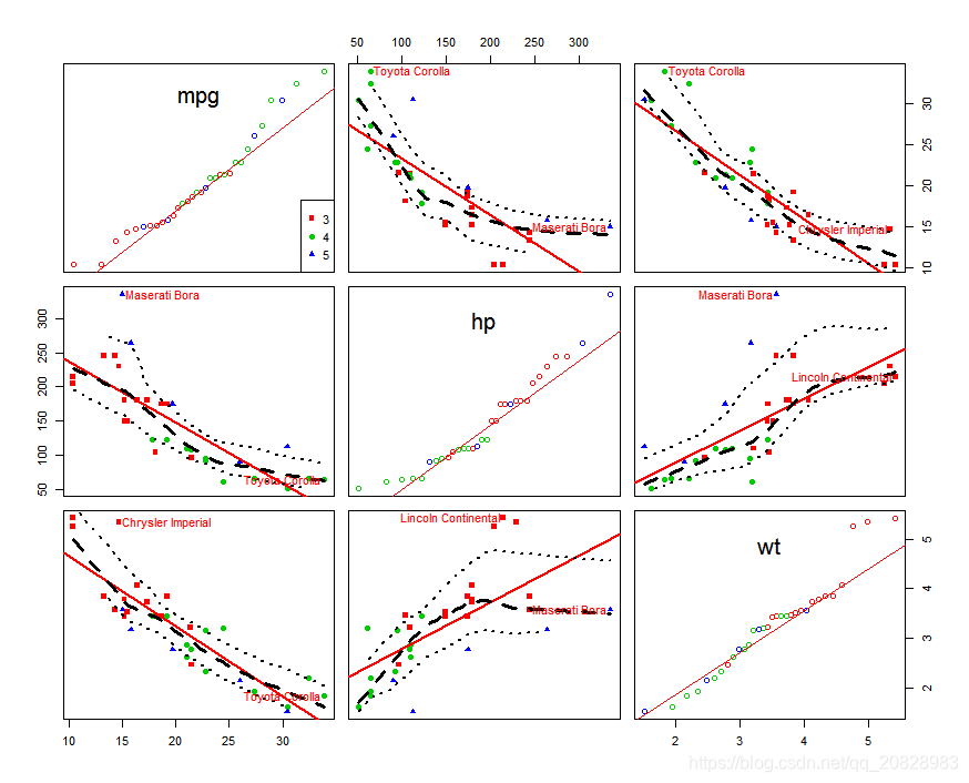
5、diagonal 对角线参数设置

可依次取为;

diagonal=list(method="adaptiveDensity", bw=bw.nrd0, adjust=1, kernel=dnorm, na.rm=TRUE) #核密度图
diagonal=list(method="density", bw="nrd0", adjust=1, kernel="gaussian", na.rm=TRUE) #非自适应核密度估计
diagonal=list(method ="histogram", breaks="FD") #直方图忽略分组
diagonal=list(method="boxplot") #箱线图
diagonal=list(method="qqplot") #normal QQ plot QQ图
diagonal=list(method="oned") #倾斜于对角线的地毯图

#核密度图
car::scatterplotMatrix(mtcars[c("mpg", "hp", "wt")],
smooth = list(spread = T, col.smooth = "black", col.spread = "black", lty.smooth=2, lwd.smooth=3, lty.spread=3, lwd.spread=2),
id = T, groups = mtcars$gear, by.groups = F,
pch = c(15,16,17),col = c("red", "green3", "blue"),
diagonal=list(method="adaptiveDensity", bw=bw.nrd0, adjust=1, kernel=dnorm, na.rm=TRUE) )
#非自适应核密度估计
car::scatterplotMatrix(mtcars[c("mpg", "hp", "wt")],
smooth = list(spread = T, col.smooth = "black", col.spread = "black", lty.smooth=2, lwd.smooth=3, lty.spread=3, lwd.spread=2),
id = T, groups = mtcars$gear, by.groups = F,
pch = c(15,16,17),col = c("red", "green3", "blue"),
diagonal=list(method="density", bw="nrd0", adjust=1, kernel="gaussian", na.rm=TRUE) )
#直方图忽略分组
car::scatterplotMatrix(mtcars[c("mpg", "hp", "wt")],
smooth = list(spread = T, col.smooth = "black", col.spread = "black", lty.smooth=2, lwd.smooth=3, lty.spread=3, lwd.spread=2),
id = T, groups = mtcars$gear, by.groups = F,
pch = c(15,16,17),col = c("red", "green3", "blue"),
diagonal=list(method ="histogram", breaks="FD") )
#箱线图
car::scatterplotMatrix(mtcars[c("mpg", "hp", "wt")],
smooth = list(spread = T, col.smooth = "black", col.spread = "black", lty.smooth=2, lwd.smooth=3, lty.spread=3, lwd.spread=2),
id = T, groups = mtcars$gear, by.groups = F,
pch = c(15,16,17),col = c("red", "green3", "blue"),
diagonal=list(method="boxplot"))
#normal QQ plot QQ图
car::scatterplotMatrix(mtcars[c("mpg", "hp", "wt")],
smooth = list(spread = T, col.smooth = "black", col.spread = "black", lty.smooth=2, lwd.smooth=3, lty.spread=3, lwd.spread=2),
id = T, groups = mtcars$gear, by.groups = F,
pch = c(15,16,17),col = c("red", "green3", "blue"),
diagonal=list(method="qqplot") )
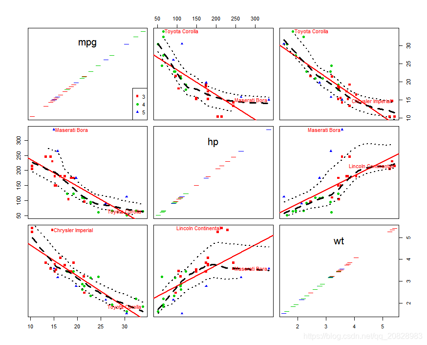
#倾斜于对角线的地毯图
car::scatterplotMatrix(mtcars[c("mpg", "hp", "wt")],
smooth = list(spread = T, col.smooth = "black", col.spread = "black", lty.smooth=2, lwd.smooth=3, lty.spread=3, lwd.spread=2),
id = T, groups = mtcars$gear, by.groups = F,
pch = c(15,16,17),col = c("red", "green3", "blue"),
diagonal=list(method="oned") )

图依次是：

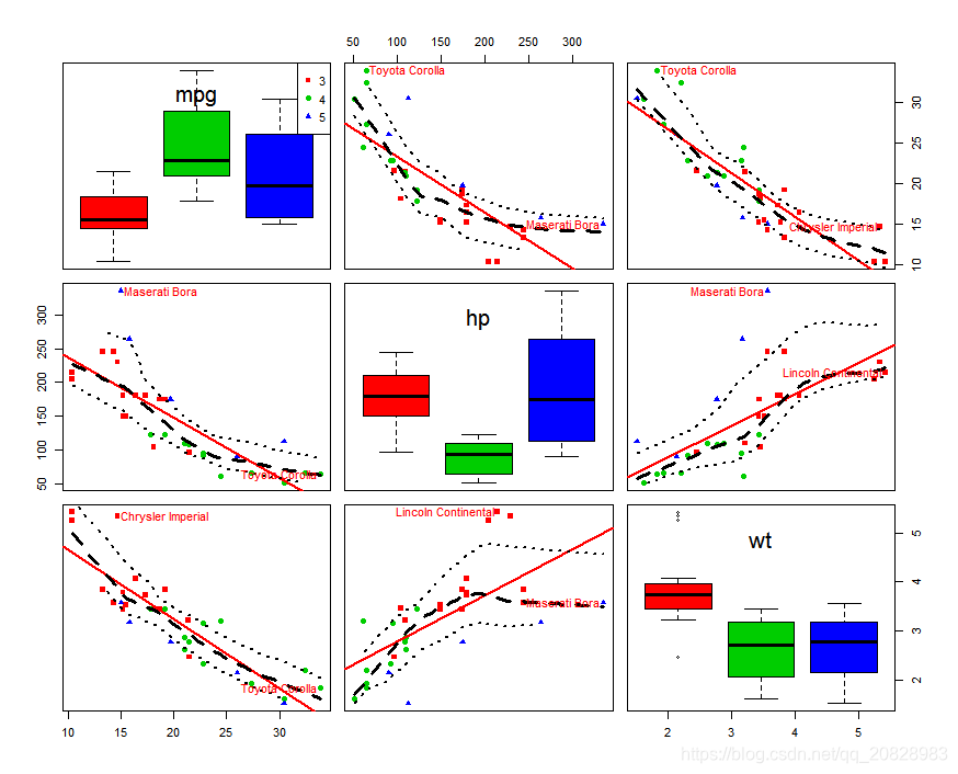
6、legend 图例

legend 参数是我花费时间最多的，百度不到相关说明，help帮助英文看了也很疑惑，使用不来。最终下了car报源码，自己看了才明白，可以调整其在第一个对角线图形中的位置。如：legend = list(coords= "topleft") （左上角）

位置有9个选择：

c("bottomright", "bottom", "bottomleft", "left", "topleft", "top", "topright", "right", "center")

car::scatterplotMatrix(mtcars[c("mpg", "hp", "wt")],
smooth = list(spread = T, col.smooth = "black", col.spread = "black", lty.smooth=2, lwd.smooth=3, lty.spread=3, lwd.spread=2),
id = T, groups = mtcars$gear, by.groups = F,
pch = c(15,16,17),col = c("red", "green3", "blue"),
diagonal=list(method="boxplot"),
legend = list(coords= "topleft"))

附scatterplotMatrix函数源码：

# fancy scatterplot matrices (J. Fox)
# 2010-09-04: J. Fox: changed color choice
# 2010-09-16: fixed point color when col is length 1
# 2011-03-08: J. Fox: changed col argument
# 2012-04-18: J. Fox: fixed labels argument in scatterplotMatrix.formula()
# 2012-09-12: J. Fox: smoother now given as function
# 2012-09-19: J. Fox: restored smooth and span args for backwards compatibility
# 2013-02-08: S. Weisberg: bug-fix for showLabels with groups
# 2013-08-26: J. Fox: added use argument
# 2014-08-07: J. Fox: plot univariate distributions by group (except for histogram)
# 2014-08-17: J. Fox: report warning rather than error if not enough points in a group
# to compute density
# 2014-09-04: J. Fox: empty groups produce warning rather than error
# 2017-02-14: J. Fox: consolidated smooth, id, legend, and ellipse arguments
# 2017-02-17: S. Weisberg, more changes to arguments
# 2017-02-19: J. Fox: bug fixes and improvement to col argument
# 2017-04-18; S. Weisberg fixed bug in handling id=FALSE with matrix/data frame input.
# 2017-04-18; S. Weisberg changed the default for by.groups to TRUE
# 2017-04-20: S. Weisberg fixed bug with color handling
# 2017-04-20: S. Weisberg the default diagonal is now adaptiveDensity using adaptiveKernel fn
# diagonal argument is now a list similar to regLine and smooth
# changed arguments and updated man page
# 2017-05-08: S. Weisberg changed col=carPalette()
# 2017-06-22: J. Fox: eliminated extraneous code for defunct labels argument; small cleanup
# 2017-12-07: J. Fox: added fill, fill.alpha subargs to ellipse arg, suggestion of Michael Friendly.
# 2018-02-09: S. Weisberg removed the transform and family arguments from the default method
# 2018-04-02: J. Fox: warning rather than error for too few colors.
# 2018-04-12: J. Fox: clean up handling of groups arg.
scatterplotMatrix <- function(x, ...){
UseMethod("scatterplotMatrix")
}
scatterplotMatrix.formula <- function (formula, data=NULL, subset, ...) {
na.save <- options(na.action=na.omit)
on.exit(options(na.save))
na.pass <- function(dframe) dframe
m <- match.call(expand.dots = FALSE)
if (is.matrix(eval(m$data, sys.frame(sys.parent()))))
m$data <- as.data.frame(data)
m$id <- m$formula <- m$... <- NULL
m$na.action <- na.pass
m[[1]] <- as.name("model.frame")
if (!inherits(formula, "formula") | length(formula) != 2)
stop("invalid formula")
rhs <- formula[[2]]
if ("|" != deparse(rhs[[1]])){
groups <- FALSE
}
else{
groups <- TRUE
formula <- as.character(formula)
formula <- as.formula(sub("\\|", "+", formula))
}
m$formula <-formula
if (missing(data)){
X <- na.omit(eval(m, parent.frame()))
# if (is.null(labels)) labels <- gsub("X", "", row.names(X))
}
else{
X <- eval(m, parent.frame())
# if (is.null(labels)) labels <- rownames(X)
}
if (!groups) scatterplotMatrix(X, ...)
else{
ncol<-ncol(X)
scatterplotMatrix.default(X[, -ncol], groups=X[, ncol], ...)
}
}
scatterplotMatrix.default <-
function(x, smooth=TRUE, id=FALSE, legend=TRUE,
regLine=TRUE, ellipse=FALSE,
var.labels=colnames(x),
diagonal=TRUE,
plot.points=TRUE,
groups=NULL, by.groups=TRUE,
use=c("complete.obs", "pairwise.complete.obs"),
col=carPalette()[-1],
pch=1:n.groups,
cex=par("cex"), cex.axis=par("cex.axis"),
cex.labels=NULL, cex.main=par("cex.main"), row1attop=TRUE, ...){
transform <- FALSE
# family <- "bcPower"
force(col)
# n.groups <- if(by.groups) length(levels(groups)) else 1
if(isFALSE(diagonal)) diagonal <- "none" else {
diagonal.args <- applyDefaults(diagonal, defaults=list(method="adaptiveDensity"), type="diag")
diagonal <- if(!isFALSE(diagonal.args)) diagonal.args$method
diagonal.args$method <- NULL
}
# regLine; use old arguments reg.line, lty and lwd
regLine.args <- applyDefaults(regLine, defaults=list(method=lm, lty=1, lwd=2,
col=col), type="regLine")
if(!isFALSE(regLine.args)) {
reg.line <- regLine.args$method
lty <- regLine.args$lty
lwd <- regLine.args$lwd
} else reg.line <- "none"
# setup smoother, now including spread
n.groups <- if(is.null(groups)) 1
else {
if (!is.factor(groups)) groups <- as.factor(groups)
length(levels(groups))
}
smoother.args <- applyDefaults(smooth, defaults=list(smoother=loessLine,
spread=(n.groups)==1, col=col, lty.smooth=2, lty.spread=4), type="smooth")
if (!isFALSE(smoother.args)) {
# check for an argument 'var' in smoother.args.
if(!is.null(smoother.args$var)) smoother.args$spread <- smoother.args$var
# end change
smoother <- smoother.args$smoother
spread <- if(is.null(smoother.args$spread)) TRUE else smoother.args$spread
smoother.args$spread <- smoother.args$smoother <- NULL
if(n.groups==1) smoother.args$col <- col[1]
}
else smoother <- "none"
# setup id
id <- applyDefaults(id, defaults=list(method="mahal", n=2, cex=1, col=col, location="lr"), type="id")
if (is.list(id) && "identify" %in% id$method) stop("interactive point identification not permitted")
if (isFALSE(id)){
id.n <- 0
id.method <- "mahal"
labels <- id.cex <- id.col <- id.location <- NULL
}
else{
labels <- if(!is.null(id$labels)) id$labels else row.names(x)
id.method <- id$method
id.n <- id$n
id.cex <- id$cex
id.col <- id$col
id.location <- id$location
}
if (is.null(labels)) labels <- as.character(seq(length.out=nrow(x)))
legend <- applyDefaults(legend, defaults=list(coords=NULL), type="legend")
if (!(isFALSE(legend) || missing(groups))){
legend.plot <- TRUE
legend.pos <- legend$coords
}
else {
legend.plot <- FALSE
legend.pos <- NULL
}
# ellipse
ellipse <- applyDefaults(ellipse, defaults=list(levels=c(0.5, 0.95), robust=TRUE, fill=TRUE, fill.alpha=0.2), type="ellipse")
if (isFALSE(ellipse)){
levels <- NULL
robust <- NULL
}
else{
levels <- ellipse$levels
robust <- ellipse$robust
fill <- ellipse$fill
fill.alpha <- ellipse$fill.alpha
ellipse <- TRUE
}
# pre 2017 code follows
# family <- match.arg(family)
use <- match.arg(use)
na.action <- if (use == "complete.obs") na.omit else na.pass
if (!(missing(groups))){
x <- na.action(data.frame(groups, labels, x, stringsAsFactors=FALSE))
# groups <- as.factor(as.character(x[, 1]))
groups <- x$groups
# if (!is.factor(groups)) groups <- as.factor(as.character(x[,1]))
labels <- x[, 2]
x <- x[, -(1:2)]
}
else {
x <- na.action(data.frame(labels, x, stringsAsFactors=FALSE))
labels <- x[, 1]
x <- x[, -1]
id.col <- id.col[1]
}
legendPlot <- function(position="topright"){
usr <- par("usr")
legend(position, bg="white",
legend=levels(groups), pch=pch, col=col[1:n.groups],
cex=cex)
}
do.legend <- legend.plot
####### diagonal panel functions
# The following panel function adapted from Richard Heiberger
panel.adaptiveDensity <- function(x, ...){
args <- applyDefaults(diagonal.args,
defaults=list(bw=bw.nrd0, adjust=1, kernel=dnorm, na.rm=TRUE))
if (n.groups > 1){
levs <- levels(groups)
for (i in 1:n.groups){
xx <- x[levs[i] == groups]
dens.x <- try(adaptiveKernel(xx, adjust = args$adjust, na.rm=args$na.rm,
bw=args$bw, kernel=args$kernel), silent=TRUE)
if (!inherits(dens.x, "try-error")){
lines(dens.x$x, min(x, na.rm=TRUE) + dens.x$y *
diff(range(x, na.rm=TRUE))/diff(range(dens.x$y, na.rm=TRUE)), col=col[i])
}
else warning("cannot estimate density for group ", levs[i], "\n",
dens.x, "\n")
rug(xx, col=col[i])
}
}
else {
dens.x <- adaptiveKernel(x, adjust = args$adjust, na.rm=args$na.rm,
bw=args$bw, kernel=args$kernel)
lines(dens.x$x, min(x, na.rm=TRUE) + dens.x$y * diff(range(x, na.rm=TRUE))/diff(range(dens.x$y, na.rm=TRUE)), col=col[1])
rug(x)
}
if (do.legend) legendPlot(position=if (is.null(legend.pos)) "topright" else legend.pos)
do.legend <<- FALSE
}
#
panel.density <- function(x, ...){
args <- applyDefaults(diagonal.args,
defaults=list(bw="nrd0", adjust=1, kernel="gaussian", na.rm=TRUE))
if (n.groups > 1){
levs <- levels(groups)
for (i in 1:n.groups){
xx <- x[levs[i] == groups]
dens.x <- try(density(xx, adjust = args$adjust, na.rm=args$na.rm,
bw=args$bw, kernel=args$kernel), silent=TRUE)
if (!inherits(dens.x, "try-error")){
lines(dens.x$x, min(x, na.rm=TRUE) + dens.x$y *
diff(range(x, na.rm=TRUE))/diff(range(dens.x$y, na.rm=TRUE)), col=col[i])
}
else warning("cannot estimate density for group ", levs[i], "\n",
dens.x, "\n")
rug(xx, col=col[i])
}
}
else {
dens.x <- density(x, adjust = args$adjust, na.rm=args$na.rm,
bw=args$bw, kernel=args$kernel)
lines(dens.x$x, min(x, na.rm=TRUE) + dens.x$y * diff(range(x, na.rm=TRUE))/diff(range(dens.x$y, na.rm=TRUE)), col=col[1])
rug(x)
}
if (do.legend) legendPlot(position=if (is.null(legend.pos)) "topright" else legend.pos)
do.legend <<- FALSE
}
panel.histogram <- function(x, ...){
par(new=TRUE)
args <- applyDefaults(diagonal.args, defaults=list(breaks="FD"))
h.col <- col[1]
if (h.col == "black") h.col <- "gray"
hist(x, main="", axes=FALSE, breaks=args$breaks, col=h.col)
if (do.legend) legendPlot(position=if (is.null(legend.pos)) "topright" else legend.pos)
do.legend <<- FALSE
}
panel.boxplot <- function(x, ...){
b.col <- col[1:n.groups]
b.col[b.col == "black"] <- "gray"
par(new=TRUE)
if (n.groups == 1) boxplot(x, axes=FALSE, main="", col=col[1])
else boxplot(x ~ groups, axes=FALSE, main="", col=b.col)
if (do.legend) legendPlot(position=if (is.null(legend.pos)) "topright" else legend.pos)
do.legend <<- FALSE
}
# The following panel function adapted from Richard Heiberger
panel.oned <- function(x, ...) {
range <- range(x, na.rm=TRUE)
delta <- diff(range)/50
y <- mean(range)
if (n.groups == 1) segments(x - delta, x, x + delta, x, col = col[1])
else {
segments(x - delta, x, x + delta, x, col = col[as.numeric(groups)])
}
if (do.legend) legendPlot(position=if (is.null(legend.pos)) "bottomright" else legend.pos)
do.legend <<- FALSE
}
panel.qqplot <- function(x, ...){
par(new=TRUE)
if (n.groups == 1) qqnorm(x, axes=FALSE, xlab="", ylab="", main="", col=col[1])
else qqnorm(x, axes=FALSE, xlab="", ylab="", main="", col=col[as.numeric(groups)])
qqline(x, col=col[1])
if (do.legend) legendPlot(position=if (is.null(legend.pos)) "bottomright" else legend.pos)
do.legend <<- FALSE
}
panel.blank <- function(x, ...){
if (do.legend) legendPlot(if (is.null(legend.pos)) "topright" else legend.pos)
do.legend <<- FALSE
}
which.fn <- match(diagonal,
c("adaptiveDensity", "density", "boxplot", "histogram", "oned", "qqplot", "none"))
if(is.na(which.fn)) stop("incorrect name for the diagonal argument, see ?scatterplotMatrix")
diag <- list(panel.adaptiveDensity, panel.density, panel.boxplot, panel.histogram, panel.oned,
panel.qqplot, panel.blank)[[which.fn]]
groups <- as.factor(if(missing(groups)) rep(1, length(x[, 1])) else groups)
counts <- table(groups)
if (any(counts == 0)){
levels <- levels(groups)
warning("the following groups are empty: ", paste(levels[counts == 0], collapse=", "))
groups <- factor(groups, levels=levels[counts > 0])
}
# n.groups <- length(levels(groups))
if (n.groups > length(col)) {
warning("number of groups exceeds number of available colors\n colors are recycled")
col <- rep(col, n.groups)
}
if (length(col) == 1) col <- rep(col, 3)
labs <- labels
pairs(x, labels=var.labels,
cex.axis=cex.axis, cex.main=cex.main, cex.labels=cex.labels, cex=cex,
diag.panel=diag, row1attop = row1attop,
panel=function(x, y, ...){
for (i in 1:n.groups){
subs <- groups == levels(groups)[i]
if (plot.points) points(x[subs], y[subs], pch=pch[i], col=col[if (n.groups == 1) 1 else i], cex=cex)
if (by.groups){
if (is.function(smoother)) smoother(x[subs], y[subs], col=smoother.args$col[i],
log.x=FALSE, log.y=FALSE, spread=spread, smoother.args=smoother.args)
if (is.function(reg.line)) regLine(reg.line(y[subs] ~ x[subs]), lty=lty, lwd=lwd, col=regLine.args$col[i])
if (ellipse) dataEllipse(x[subs], y[subs], plot.points=FALSE,
levels=levels, col=col[i], robust=robust, lwd=1,
fill=fill, fill.alpha=fill.alpha)
showLabels(x[subs], y[subs], labs[subs], method=id.method,
n=id.n, col=col[i], cex=id.cex, location=id.location,
all=list(labels=labs, subs=subs))
}
}
if (!by.groups){
if (is.function(reg.line)) abline(reg.line(y ~ x), lty=lty, lwd=lwd, col=regLine.args$col[1])
if (is.function(smoother)) smoother(x, y, col=col[1],
log.x=FALSE, log.y=FALSE, spread=spread, smoother.args=smoother.args)
if (ellipse) dataEllipse(x, y, plot.points=FALSE, levels=levels, col=smoother.args$col,
robust=robust, lwd=1, fill=fill, fill.alpha=fill.alpha)
showLabels(x, y, labs, method=id.method,
n=id.n, col=id.col, location=id.location, cex=id.cex)
}
}, ...
)
}
spm <- function(x, ...){
scatterplotMatrix(x, ...)
}

weixin_43230383

关注

7
点赞
踩
20

收藏

觉得还不错? 一键收藏
0
评论
car::scatterplotmatrix散点图矩阵参数详解

转载自：https://blog.csdn.net/qq_20828983/article/details/95659791在R语言实战第二版书，第八章回归分析时，用到了scatterplotmatrix函数绘制散点图矩阵，发现已经不是当前最新的car包了，函数参数都错误了。在网上百度发现基本没有关于此函数的详细介绍，只有自己动手，查看help了。趁热打铁，写个说明。基于的car版本为：3.0-3目录一睹为快1、数据添加2、smooth 参数3、id 控制点标识4、grou.
复制链接

扫一扫