


目录
背景
断断续续学习yolo已经一个月了,虽然目前还是感觉一知半解,但是觉得有必要从今天开始写一篇博客来记录之前的使用经过,以及更加深刻的对于yolo3的认知,我已预感到此篇博客篇幅一定过长。不过内心还是有一丝小激动的。
一开始是由于需要做图像的分类并且要画框框也就是定位,由于是视频源,rtsp协议要求具有实时性,也要具有准确性,于是,yolo当之无愧成为了我的选择。
在一开始我选择了使用python进行算法的开发,在python+tensorflow下,有一套前辈写好的yolo模型。在此附上链接:https://github.com/qqwweee/keras-yolo3
前边会更多设计理论知识以及自己的推敲,后边会有代码的详解,我会从yolo的第一代开始说起。
yolov1之前的RCNN系列目标检测算法,其本质仍是一个分类问题,基本思路是通过滑窗在图像上滑动,遍历完整个图像,分别判断窗口图像的分类,再通过回归方法调整物体精确边框,达到检测和定位的目的。其后改进的fast-RCNN系列在速度上做了提升,基本流程是先通过CNN生成大量的region proposal,即潜在的目标区域,再用另一个CNN去提取该潜在目标区域的特征,进行类别判断。
与RCNN的先定位出潜在位置,再判断分类不同,YOLO v1是一个端到端的目标检测算法,通过一个CNN网络就可以输出物体的类别以及物体的位置(还有类别的置信度)。相较于其他先进的物体检测系统,YOLO的物体定位精度略低,对小物体的检测效果不太好,但是在背景上预测出不存在的物体(false positives)的情况会少一些。
YOLO检测简易流程:
1.将图像resize到448 * 448作为神经网络的输入
2.运行神经网络,得到一些bounding box坐标位置、物体的置信度和20个类别概率
3.进行非极大值抑制,筛选Boxes
YOLOv1
YOLOv1简介
相比之前的目标检测算法,YOLO结构简单,端到端,不需要预先提取region proposal,不存在重叠区域反复预判的情况,所以YOLO最大的优点就是检测快速。
YOLO v1首先将图片resize到448*448(是Imagenet224×224的2倍),再将图像分割成7*7个小网格,每个网络会输出:
1. 2个bounding box。这个bounding box包含5个值,分别是检测到的物体的中心点坐标x和y,物体的宽度和高度W、H,还有一个置信度参数C(当前box中属于某一类的概率)
2. 当前网格整体上属于哪个分类的概率,取前20个分类的概率
所以每张图片经过YOLO的CNN后的最终输出是7*7*(2*5+20)=7*7*30维的Tensor向量,如下图所示:
YOLO v1的网络结构与GoogLeNet的网络结构类似,但没有使用GoogLeNet的inception modules,而是用1*1+3*3的卷积核的组合来代替,整个YOLOv1网络结构包含24个卷积层和2个全连接层,网络的最终输出是 7*7*30维的Tensor。结构图如下:
YOLO在获取到的7*7*30维向量的基础上,根据每个小框的类别概率、每个小框的相对位置、小框内物体所属的分类以及分类置信度等信息综合判断,预测出图片上物体的位置、类别以及相应的概率,这个过程的示意图如下:


如果在grid cell里没有物体存在,则Pr(object)=0,存在的意思是指物体的ground truth中心点在这个cell里面。另外我们发现,一个grid cell里面虽然有两个Bounding Box, 但是它们共享同一组分类概率,因此同一个cell只能识别同一个物体。
边界框的大小和位置用4个值来表示:(x, y, w, h), 其中(x,y)是边界框的中心坐标,w和h是边界框的宽与高。(x, y)是相对于每个单元格左上角坐标点偏移值,并且单位是相对于单元格大小的,而w和h预测值是相对于整个图片的宽和高的比例,这样理论上4个元素的大小在[0, 1]范围内,而且每个边界框的预测值实际上包含5个元素:(x, y, w, h, c)。前四个元素表征边界框的大小和位置,最后一个值是置信度。
YOLOv1训练
YOLO的训练分成两部分,先是物体的分类识别训练,再是物体的检测定位训练。
首先使用YOLO网络的前20层卷积层,加上一个平均池化层和一个全连接层,组成一个预训练网络,在ImageNet数据集上(图像尺寸:224×224)训练1000个类别的分类识别网络,最终达到Top-5精度88%,与GoogleNet的精度相当。
之后取该预训练网络的前20层,加上YOLO网络的后4个卷积层和2个全连接层,组成识别+检测定位网络,在PASCAL VOC2007数据集上(图像尺寸:448×448,含训练图片5011张,测试图片4952幅张,共包含20个种类)训练。网络最终的输出包括物体的Bounding box位置坐标信息(X,Y,W,H)和类别概率,将值归一化到[0,1],使用Leaky Relu作为激活函数,并在第一个全连接层后接了一个ratio=0.5的Dropout 层,以防止过拟合。
损失函数

YOLO的损失函数包含3部分,分别是位置坐标损失函数,置信度损失函数和类别预测损失函数(注意置信度跟类别预测的区别,置信度是7×7个小区域里预测出来2个分类的置信度,共有7×7×2个,类别预测是7×7个小区域整体上分别属于20个类别的概率,共有7×7×20。那么为什么不干脆只记录每个小区域所属的最大概率对应的类别呢,这样是不是数据维度是7×7×1就ok了?这是为了在最后做整体上的综合整合),如何在这3部分损失函数之间找到一个平衡点,YOLO主要从以下几个方面考虑:
1. 坐标损失函数方面,每个小区域上输出的8维位置坐标偏差的权重应该比20维类别预测偏差的权重要大,因为首先从体量上考虑,20维的影响很容易超过8维的影响,导致分类准确但是位置偏差过大,再者最后还会在整体的分类预测结果上综合判断物体的类别,所以单个小区域的分类误差稍微大一点不至于影响最终的结果。最终设置位置坐标损失和类别损失函数的权重比为5:1
2. 置信度损失函数方面,在不含有目标物体的网格上,物体的置信度是0,并且图像上大部分区域都是不含目标物体的,这些过多的置信度为0对梯度的贡献会远远大于含目标物体的网格对梯度的贡献,这就容易导致网络不稳定或者发散,也就是说网络会倾向于预测每个小网格不含有物体,因为大部分情况下这种预测都是正确的。所以需要减弱不含目标物体的网格的贡献,取权重系数为0.5,含目标物体的网格的权重正常取1
3. 目标物体大小不等方面,考虑到目标物体有大有小,对于大的物体,坐标预测存在一些偏差无伤大雅,但是对于小的目标物体,偏差一点可能就是另外一个东西了。为了解决这个问题,作者将位置坐标的W和H分别取平方根来代替原本的W和H,以达到值越小,对同等大小改变的相应越大的目的,对于这一点,可以从下图上更直观的看出来:
上图中可见对于水平方向上同等尺度的增量,基准值越小,其在平方根上产生的偏差就越大,如图中的绿色段明显大于红色段。
基于以上3点考虑,YOLO综合的损失函数可以总结如下图:

训练出来的网络再对预测定位结果进行一个非极大值抑制,就可以完美定位出物体的位置了。
YOLOv1测试
输入图片,网络会按照与训练时相同的分割方式将测试图片分割成S x S的形状,因此,划分出来的每个网格预测的class信息和Bounding box预测的confidence信息相乘,就得到了每个Bounding box的class-specific confidence score,即得到了每个Bounding box预测具体物体的概率和位置重叠的概率。
对于98个Bounding Box都这么运算,最后可以得到:

每个“条”一共有20个值,分别是20个物体的得分,因此一共有98*20个值,我们按照类别把它们分为20类。之后的过程如下(先以第一类假设为“dog”举例):


直观来感受一下非极大值抑制的过程:


YOLOv2
YOLOv2用的是Darknet-19网络用于特征提取的。作者在论文中这样说到:其实很多检测框架都是依赖于VGG-16网络来提取特征的,VGG-16是一个强大的,准确率高的分类网络,但是它很复杂。看没看到,作者用了一个“但是”就把这个网络否定了,然后自己牛逼的提出了一个比它优秀的网络。作者继续补刀:仅一张分辨率为224*224的图片在单次传递的时候,VGG-16的卷积层就需要30.69 billion次浮点运算操作。看一张网络运算浮点操作的图就知道了,反正你知道VGG-16运算量很大就行了。
看一下Darknet-19的结构:

再详细看一下在Darknet-19的基础上的YOLOv2网络结构

YOLOv2网络中第23层上面是Darknet-19网络,后面是添加的检测网络。
YOLOv2采用神经网络结构,有32层。结构比较常规,包含一些卷积和最大池化,其中有一些1*1卷积,采用GoogLeNet一些微观的结构。其中要留意的是,第25层和28层有一个route。例如第28层的route是27和24,即把27层和24层合并到一起输出到下一层,route层的作用是进行层的合并。30层输出的大小是13*13,是指把图片通过卷积或池化,最后缩小到一个13*13大小的格。每一个格子的output参数是125。所以最后输出的参数一共是13*13*125
关于YOLOv2 边框预测计算:
上面说了最后输出参数是13*13*125, 是因为一共有13*13个格子,每个格子预测出5个bounding box,每个bounding box预测25个数,其中20个是class的probability,其余5个参数中有四个表示stx、sty、tw、th,这4个来识别边框的位置和大小,还有1个数是confidence,表示边框预测里有真正的对象的概率,所以一共是13*13*125个数。接下来看一下四个参数stx、sty、tw、th,是如何预测框的位置的。
这里先介绍一个anchor boxes 概念,这个悲伤的故事来源于Faster RCNN,因为faster RCNN为了不让算法漫无目的的去猜测那些目标的边框大小,于是就自己预先在每个位置上产生一定长宽比例的方框,以减少搜索量,这个方框就叫做anchor boxes,anchor的意思是“锚”,“固定”的意思,大多数人是把这个解释为“锚”,不过我觉得解释成“固定”比较好,其实也有锚的意思,因为这个是相对于中心点来说的,就是在中心点的周围产生几个固定比例的边框,所以这个“中心点”就把这几个框给锚住了,他们共用一个中心点,(当然在YOLOv2中这个中心点是一个格子的大小,所以会在格子里微小移动)。
faster RCNN在每个位置上产生了9个不同长宽比例的anchor boxes ,这几种比例以及比例的种数作者认为不合理,是手动选出来的,虽然网络最终可以学出来,但如果我们可以给出更好的anchor,那么网络肯定更加容易训练而且效果更好。
于是作者灵光一闪,通过K-Means聚类的方式在训练集中聚出了好的anchor模板。经过分析,确定了anchor boxes的个数以及比例。如下图
上图的左边可以看出,有5中类型的长宽比例。后面预测出stx、sty、tw、th,四个参数,再根据上图右边的计算就可以计算出预测出的box大小了,注意!上图右边里面的σ(tx)可以理解为stx,σ(ty)可以理解为sty。每一个输出的bbox是针对于一个特定的anchor,anchor其实是bbox的width及height的一个参考。pw和ph是某个anchor box的宽和高,一个格子的Cx和Cy单位都是1,σ(tx),σ(ty)是相对于某个格子左上角的偏移量。
这个地方不是很好理解,我举个例子,比如说我预测出了stx、sty、tw、th四个参数分别是0.2,0.1,0.2,0.32,row:1,col:1假如anchor比例取:w:3.19275,h:4.00944,这其中row和col就是锚点相对于整个网格的偏移的格子数,在这个偏移量的基础上计算格子中心位置,
计算出:
bx=0.2+1=1.2
by=0.1+1=1.1
bw=3.19275*exp(0.2)=3.89963
bh=4.00944*exp(0.32)=5.52151
然后分别将这些归一化(同除以13),得:bx=0.09,by=0.08,bw=0.30,bh=0.42.具体是否要输出当前的边框,它的概率,还有生成的物体的类别,这个取决于后面的probability和confidence
YOLOv2所带来的改变
结合yolov2的论文来讨论。
主要包括三个部分:Better,Faster,Stronger,其中前面两部分基本上讲的是YOLOv2,最后一部分讲的是YOLO9000。(YOLO9000这里暂时不讲)
Better
这部分细节很多,想要详细了解的话建议还是看源码。
很明显,本篇论文是YOLO作者为了改进原有的YOLO算法所写的。YOLO有两个缺点:一个缺点在于定位不准确,另一个缺点在于和基于region proposal的方法相比召回率较低。因此YOLOv2主要是要在这两方面做提升。另外YOLOv2并不是通过加深或加宽网络达到效果提升,反而是简化了网络。大概看一下YOLOv2的表现:YOLOv2算法在VOC 2007数据集上的表现为67 FPS时,MAP为76.8,在40FPS时,MAP为78.6.
1.Batch Normalization
BN(Batch Normalization)层简单讲就是对网络的每一层的输入都做了归一化,这样网络就不需要每层都去学数据的分布,收敛会快点。原来的YOLO算法(采用的是GoogleNet网络提取特征)是没有BN层的,因此在YOLOv2中作者为每个卷积层都添加了BN层。另外由于BN可以规范模型,所以本文加入BN后就把dropout去掉了。实验证明添加了BN层可以提高2%的mAP。BN是详细学习可以参考:https://www.cnblogs.com/ranjiewen/articles/7748232.html,介绍的非常详细。
2.High Resolution Classifier
首先fine-tuning的作用不言而喻,现在基本跑个classification或detection的模型都不会从随机初始化所有参数开始,所以一般都是用预训练的网络来finetuning自己的网络,而且预训练的网络基本上都是在ImageNet数据集上跑的,一方面数据量大,另一方面训练时间久,而且这样的网络都可以在相应的github上找到。
原来的YOLO网络在预训练的时候采用的是224*224的输入(这是因为一般预训练的分类模型都是在ImageNet数据集上进行的),然后在detection的时候采用448*448的输入,这会导致从分类模型切换到检测模型的时候,模型还要适应图像分辨率的改变。而YOLOv2则将预训练分成两步:先用224*224的输入从头开始训练网络,大概160个epoch(表示将所有训练数据循环跑160次),然后再将输入调整到448*448,再训练10个epoch。注意这两步都是在ImageNet数据集上操作。最后再在检测的数据集上fine-tuning,也就是detection的时候用448*448的图像作为输入就可以顺利过渡了。作者的实验表明这样可以提高几乎4%的MAP。
3.Convolutional With Anchor Boxes
原来的YOLO是利用全连接层直接预测bounding box的坐标,而YOLOv2借鉴了Faster R-CNN的思想,引入anchor。首先将原网络的全连接层和最后一个pooling层去掉,使得最后的卷积层可以有更高分辨率的特征;然后缩减网络,用416*416大小的输入代替原来448*448。这样做的原因在于希望得到的特征图都有奇数大小的宽和高,奇数大小的宽和高会使得每个特征图在划分cell的时候就只有一个center cell(比如可以划分成7*7或9*9个cell,center cell只有一个,如果划分成8*8或10*10的,center cell就有4个)。为什么希望只有一个center cell呢?因为大的object一般会占据图像的中心,所以希望用一个center cell去预测,而不是4个center cell去预测。网络最终将416*416的输入变成13*13大小的feature map输出,也就是缩小比例为32。
我们知道原来的YOLO算法将输入图像分成7*7的网格,每个网格预测两个bounding box,因此一共只有98个box,但是在YOLOv2通过引入anchor boxes,预测的box数量超过了1千(以输出feature map大小为13*13为例,每个grid cell有9个anchor box的话,一共就是13*13*9=1521个,当然由后面第4点可知,最终每个grid cell选择5个anchor box)。顺便提一下在Faster RCNN在输入大小为1000*600时的boxes数量大概是6000,在SSD300中boxes数量是8732。显然增加box数量是为了提高object的定位准确率。
作者的实验证明:虽然加入anchor使得MAP值下降了一点(69.5降到69.2),但是提高了recall(81%提高到88%)。
4.Dimension Clusters
我们知道在Faster R-CNN中anchor box的大小和比例是按经验设定的,然后网络会在训练过程中调整anchor box的尺寸。但是如果一开始就能选择到合适尺寸的anchor box,那肯定可以帮助网络越好地预测detection。所以作者采用k-means的方式对训练集的bounding boxes做聚类,试图找到合适的anchor box。
另外作者发现如果采用标准的k-means(即用欧式距离来衡量差异),在box的尺寸比较大的时候其误差也更大,而我们希望的是误差和box的尺寸没有太大关系。所以通过IOU定义了如下的距离函数,使得误差和box的大小无关:
![]()
如下图Figure2,左边是聚类的簇个数核IOU的关系,两条曲线分别代表两个不同的数据集。在分析了聚类的结果并平衡了模型复杂度与recall值,作者选择了K=5,这也就是Figure2中右边的示意图是选出来的5个box的大小,这里紫色和黑色也是分别表示两个不同的数据集,可以看出其基本形状是类似的。而且发现聚类的结果和手动设置的anchor box大小差别显著。聚类的结果中多是高瘦的box,而矮胖的box数量较少。
Table1中作者采用的5种anchor(Cluster IOU)的Avg IOU是61,而采用9种Anchor Boxes的Faster RCNN的Avg IOU是60.9,也就是说本文仅选取5种box就能达到Faster RCNN的9中box的效果。

5.Direct Location prediction
作者在引入anchor box的时候遇到的第二个问题:模型不稳定,尤其是在训练刚开始的时候。作者认为这种不稳定主要来自预测box的(x,y)值。我们知道在基于region proposal的object detection算法中,是通过预测下图中的tx和ty来得到(x,y)值,也就是预测的是offset。另外关于文中的这个公式,个人认为应该把后面的减号改成加号,这样才能符合公式下面的example。这里xa和ya是anchor的坐标,wa和ha是anchor的size,x和y是坐标的预测值,tx和ty是偏移量。
在这里作者并没有采用直接预测offset的方法,还是沿用了YOLO算法中直接预测相对于grid cell的坐标位置的方式。
前面提到网络在最后一个卷积层输出13*13大小的feature map,然后每个cell预测5个bounding box,然后每个bounding box预测5个值:tx,ty,tw,th和to(这里的to类似YOLOv1中的confidence)。看下图,tx和ty经过sigmoid函数处理后范围在0到1之间,这样的归一化处理也使得模型训练更加稳定;cx和cy表示一个cell和图像左上角的横纵距离;pw和ph表示bounding box的宽高,这样bx和by就是cx和cy这个cell附近的anchor来预测tx和ty得到的结果
如果对上面的公式不理解,可以看Figure3,首先是cx和cy,表示grid cell与图像左上角的横纵坐标距离,黑色虚线框是bounding box,蓝色矩形框就是预测的结果。

6.Fine-Grained Features
这里主要是添加了一个层:passthrough layer。这个层的作用就是将前面一层的26*26的feature map和本层的13*13的feature map进行连接,有点像ResNet。这样做的原因在于虽然13*13的feature map对于预测大的object以及足够了,但是对于预测小的object就不一定有效。也容易理解,越小的object,经过层层卷积和pooling,可能到最后都不见了,所以通过合并前一层的size大一点的feature map,可以有效检测小的object。
7.Multi-Scale Training
为了让YOLOv2模型更加robust,作者引入了Muinti-Scale Training,简单讲就是在训练时输入图像的size是动态变化的,注意这一步是在检测数据集上fine tune时候采用的,不要跟前面在Imagenet数据集上的两步预训练分类模型混淆,本文细节确实很多。具体来讲,在训练网络时,每训练10个batch(文中是10个batch,个人认为会不会是笔误,不应该是10个epoch?),网络就会随机选择另一种size的输入。那么输入图像的size的变化范围要怎么定呢?前面我们知道本文网络本来的输入是416*416,最后会输出13*13的feature map,也就是说downsample的factor是32,因此作者采用32的倍数作为输入的size,具体来讲文中作者采用从{320,352,…,608}的输入尺寸。
这种网络训练方式使得相同网络可以对不同分辨率的图像做detection。虽然在输入size较大时,训练速度较慢,但同时在输入size较小时,训练速度较快,而multi-scale training又可以提高准确率,因此算是准确率和速度都取得一个不错的平衡。
Table3就是在检测时,不同输入size情况下的YOLOv2和其他object detection算法的对比。可以看出通过multi-scale training的检测模型,在测试的时候,输入图像在尺寸变化范围较大的情况下也能取得mAP和FPS的平衡。不过同时也可以看出SSD算法的表现也十分抢眼
Faster
在YOLO v1中,作者采用的训练网络是基于GooleNet,这里作者将GooleNet和VGG16做了简单的对比,GooleNet在计算复杂度上要优于VGG16(8.25 billion operation VS 30.69 billion operation),但是前者在ImageNet上的top-5准确率要稍低于后者(88% VS 90%)。而在YOLOv2中,作者采用了新的分类模型作为基础网络,那就是Darknet-19。
1.Darknet-19
Table6是最后的网络结构:Darknet-19只需要5.58 billion operation。这个网络包含19个卷积层和5个max pooling层,而在YOLOv1中采用的GooleNet,包含24个卷积层和2个全连接层,因此Darknet-19整体上卷积卷积操作比YOLOv1中用的GoogleNet要少,这是计算量减少的关键。最后用average pooling层代替全连接层进行预测。这个网络在ImageNet上取得了top-5的91.2%的准确率。
2.Training for Classification
这里的2和3部分在前面有提到,就是训练处理的小trick。这里的training for classification都是在ImageNet上进行预训练,主要分两步:
1.从头开始训练Darknet-19,数据集是ImageNet,训练160个epoch,输入图像的大小是224*224,初始学习率为0.1。另外在训练的时候采用了标准的数据增加方式比如随机裁剪,旋转以及色度,亮度的调整等。
2.再fine-tuning 网络,这时候采用448*448的输入,参数的除了epoch和learning rate改变外,其他都没变,这里learning rate改为0.001,并训练10个epoch。结果表明fine-tuning后的top-1准确率为76.5%,top-5准确率为93.3%,而如果按照原来的训练方式,Darknet-19的top-1准确率是72.9%,top-5准确率为91.2%。因此可以看出第1,2两步分别从网络结构和训练方式两方面入手提高了主网络的分类准确率。
3.Training for Detection
在前面第2步之后,就开始把网络移植到detection,并开始基于检测的数据再进行fine-tuning。首先把最后一个卷积层去掉,然后添加3个3*3的卷积层,每个卷积层有1024个filter,而且每个后面都连接一个1*1的卷积层,1*1卷积的filter个数根据需要检测的类来定。比如对于VOC数据,由于每个grid cell我们需要预测5个box,每个box有5个坐标值和20个类别值,所以每个grid cell有125个filter(与YOLOv1不同,在YOLOv1中每个grid cell有30个filter,还记得那个7*7*30的矩阵吗,而且在YOLOv1中,类别概率是由grid cell来预测的,也就是说一个grid cell对应的两个box的类别概率是一样的,但是在YOLOv2中,类别概率是属于box的,每个box对应一个类别概率,而不是由grid cell决定,因此这边每个box对应25个预测值(5个坐标加20个类别值),而在YOLOv1中一个grid cell的两个box的20个类别值是一样的)。另外作者还提到将最后一个3*3*512的卷积层和倒数第二个卷积层相连。最后作者在检测数据集上fine tune这个预训练模型160个epoch,学习率采用0.001,并且在第60和90epoch的时候将学习率除以10,weight decay采用0.0005。
YOLOv3
结构
yolo3是以darknet53为basemodel训练出来的模型。先来看看darknet53的网络结构:

再来看下改进后的yolo3:

再来一张别的老师总结的生动一些的结构图:

DBL
如图1左下角所示,也就是代码中的Darknetconv2d_BN_Leaky,是yolo_v3的基本组件。就是卷积+BN+Leaky relu。对于v3来说,BN和leaky relu已经是和卷积层不可分离的部分了(最后一层卷积除外),共同构成了最小组件。
RESN
n代表数字,有res1,res2, … ,res8等等,表示这个res_block里含有多少个res_unit。这是yolo_v3的大组件,yolo_v3开始借鉴了ResNet的残差结构,使用这种结构可以让网络结构更深(从v2的darknet-19上升到v3的darknet-53,前者没有残差结构)。对于res_block的解释,可以在图1的右下角直观看到,其基本组件也是DBL。
CONCAT
张量拼接。将darknet中间层和后面的某一层的上采样进行拼接。拼接的操作和残差层add的操作是不一样的,拼接会扩充张量的维度,而add只是直接相加不会导致张量维度的改变。
下面是流程流水线:
layer     filters    size              input                output
    0 conv     32  3 x 3 / 1   416 x 416 x   3   ->   416 x 416 x  32
    1 conv     64  3 x 3 / 2   416 x 416 x  32   ->   208 x 208 x  64
    2 conv     32  1 x 1 / 1   208 x 208 x  64   ->   208 x 208 x  32
    3 conv     64  3 x 3 / 1   208 x 208 x  32   ->   208 x 208 x  64
    4 Shortcut Layer: 1
    5 conv    128  3 x 3 / 2   208 x 208 x  64   ->   104 x 104 x 128
    6 conv     64  1 x 1 / 1   104 x 104 x 128   ->   104 x 104 x  64
    7 conv    128  3 x 3 / 1   104 x 104 x  64   ->   104 x 104 x 128
    8 Shortcut Layer: 5
    9 conv     64  1 x 1 / 1   104 x 104 x 128   ->   104 x 104 x  64
   10 conv    128  3 x 3 / 1   104 x 104 x  64   ->   104 x 104 x 128
   11 Shortcut Layer: 8
   12 conv    256  3 x 3 / 2   104 x 104 x 128   ->    52 x  52 x 256
   13 conv    128  1 x 1 / 1    52 x  52 x 256   ->    52 x  52 x 128
   14 conv    256  3 x 3 / 1    52 x  52 x 128   ->    52 x  52 x 256
   15 Shortcut Layer: 12
   16 conv    128  1 x 1 / 1    52 x  52 x 256   ->    52 x  52 x 128
   17 conv    256  3 x 3 / 1    52 x  52 x 128   ->    52 x  52 x 256
   18 Shortcut Layer: 15
   19 conv    128  1 x 1 / 1    52 x  52 x 256   ->    52 x  52 x 128
   20 conv    256  3 x 3 / 1    52 x  52 x 128   ->    52 x  52 x 256
   21 Shortcut Layer: 18
   22 conv    128  1 x 1 / 1    52 x  52 x 256   ->    52 x  52 x 128
   23 conv    256  3 x 3 / 1    52 x  52 x 128   ->    52 x  52 x 256
   24 Shortcut Layer: 21
   25 conv    128  1 x 1 / 1    52 x  52 x 256   ->    52 x  52 x 128
   26 conv    256  3 x 3 / 1    52 x  52 x 128   ->    52 x  52 x 256
   27 Shortcut Layer: 24
   28 conv    128  1 x 1 / 1    52 x  52 x 256   ->    52 x  52 x 128
   29 conv    256  3 x 3 / 1    52 x  52 x 128   ->    52 x  52 x 256
   30 Shortcut Layer: 27
   31 conv    128  1 x 1 / 1    52 x  52 x 256   ->    52 x  52 x 128
   32 conv    256  3 x 3 / 1    52 x  52 x 128   ->    52 x  52 x 256
   33 Shortcut Layer: 30
   34 conv    128  1 x 1 / 1    52 x  52 x 256   ->    52 x  52 x 128
   35 conv    256  3 x 3 / 1    52 x  52 x 128   ->    52 x  52 x 256
   36 Shortcut Layer: 33
   37 conv    512  3 x 3 / 2    52 x  52 x 256   ->    26 x  26 x 512
   38 conv    256  1 x 1 / 1    26 x  26 x 512   ->    26 x  26 x 256
   39 conv    512  3 x 3 / 1    26 x  26 x 256   ->    26 x  26 x 512
   40 Shortcut Layer: 37
   41 conv    256  1 x 1 / 1    26 x  26 x 512   ->    26 x  26 x 256
   42 conv    512  3 x 3 / 1    26 x  26 x 256   ->    26 x  26 x 512
   43 Shortcut Layer: 40
   44 conv    256  1 x 1 / 1    26 x  26 x 512   ->    26 x  26 x 256
   45 conv    512  3 x 3 / 1    26 x  26 x 256   ->    26 x  26 x 512
   46 Shortcut Layer: 43
   47 conv    256  1 x 1 / 1    26 x  26 x 512   ->    26 x  26 x 256
   48 conv    512  3 x 3 / 1    26 x  26 x 256   ->    26 x  26 x 512
   49 Shortcut Layer: 46
   50 conv    256  1 x 1 / 1    26 x  26 x 512   ->    26 x  26 x 256
   51 conv    512  3 x 3 / 1    26 x  26 x 256   ->    26 x  26 x 512
   52 Shortcut Layer: 49
   53 conv    256  1 x 1 / 1    26 x  26 x 512   ->    26 x  26 x 256
   54 conv    512  3 x 3 / 1    26 x  26 x 256   ->    26 x  26 x 512
   55 Shortcut Layer: 52
   56 conv    256  1 x 1 / 1    26 x  26 x 512   ->    26 x  26 x 256
   57 conv    512  3 x 3 / 1    26 x  26 x 256   ->    26 x  26 x 512
   58 Shortcut Layer: 55
   59 conv    256  1 x 1 / 1    26 x  26 x 512   ->    26 x  26 x 256
   60 conv    512  3 x 3 / 1    26 x  26 x 256   ->    26 x  26 x 512
   61 Shortcut Layer: 58
   62 conv   1024  3 x 3 / 2    26 x  26 x 512   ->    13 x  13 x1024
   63 conv    512  1 x 1 / 1    13 x  13 x1024   ->    13 x  13 x 512
   64 conv   1024  3 x 3 / 1    13 x  13 x 512   ->    13 x  13 x1024
   65 Shortcut Layer: 62
   66 conv    512  1 x 1 / 1    13 x  13 x1024   ->    13 x  13 x 512
   67 conv   1024  3 x 3 / 1    13 x  13 x 512   ->    13 x  13 x1024
   68 Shortcut Layer: 65
   69 conv    512  1 x 1 / 1    13 x  13 x1024   ->    13 x  13 x 512
   70 conv   1024  3 x 3 / 1    13 x  13 x 512   ->    13 x  13 x1024
   71 Shortcut Layer: 68
   72 conv    512  1 x 1 / 1    13 x  13 x1024   ->    13 x  13 x 512
   73 conv   1024  3 x 3 / 1    13 x  13 x 512   ->    13 x  13 x1024
   74 Shortcut Layer: 71
   75 conv    512  1 x 1 / 1    13 x  13 x1024   ->    13 x  13 x 512
   76 conv   1024  3 x 3 / 1    13 x  13 x 512   ->    13 x  13 x1024
   77 conv    512  1 x 1 / 1    13 x  13 x1024   ->    13 x  13 x 512
   78 conv   1024  3 x 3 / 1    13 x  13 x 512   ->    13 x  13 x1024
   79 conv    512  1 x 1 / 1    13 x  13 x1024   ->    13 x  13 x 512
   80 conv   1024  3 x 3 / 1    13 x  13 x 512   ->    13 x  13 x1024
   81 conv     18  1 x 1 / 1    13 x  13 x1024   ->    13 x  13 x  18
   82 detection
   83 route  79
   84 conv    256  1 x 1 / 1    13 x  13 x 512   ->    13 x  13 x 256
   85 upsample            2x    13 x  13 x 256   ->    26 x  26 x 256
   86 route  85 61
   87 conv    256  1 x 1 / 1    26 x  26 x 768   ->    26 x  26 x 256
   88 conv    512  3 x 3 / 1    26 x  26 x 256   ->    26 x  26 x 512
   89 conv    256  1 x 1 / 1    26 x  26 x 512   ->    26 x  26 x 256
   90 conv    512  3 x 3 / 1    26 x  26 x 256   ->    26 x  26 x 512
   91 conv    256  1 x 1 / 1    26 x  26 x 512   ->    26 x  26 x 256
   92 conv    512  3 x 3 / 1    26 x  26 x 256   ->    26 x  26 x 512
   93 conv     18  1 x 1 / 1    26 x  26 x 512   ->    26 x  26 x  18
   94 detection
   95 route  91
   96 conv    128  1 x 1 / 1    26 x  26 x 256   ->    26 x  26 x 128
   97 upsample            2x    26 x  26 x 128   ->    52 x  52 x 128
   98 route  97 36
   99 conv    128  1 x 1 / 1    52 x  52 x 384   ->    52 x  52 x 128
  100 conv    256  3 x 3 / 1    52 x  52 x 128   ->    52 x  52 x 256
  101 conv    128  1 x 1 / 1    52 x  52 x 256   ->    52 x  52 x 128
  102 conv    256  3 x 3 / 1    52 x  52 x 128   ->    52 x  52 x 256
  103 conv    128  1 x 1 / 1    52 x  52 x 256   ->    52 x  52 x 128
  104 conv    256  3 x 3 / 1    52 x  52 x 128   ->    52 x  52 x 256
  105 conv     18  1 x 1 / 1    52 x  52 x 256   ->    52 x  52 x  18
  106 detection
这么多图,就是为了熟悉流程,这对后边看代码非常的重要。
对于代码层面的layers数量一共有252层,包括add层23层(主要用于res_block的构成,每个res_unit需要一个add层,一共有1+2+8+8+4=23层)。除此之外,BN层和LeakyReLU层数量完全一样(72层),在网络结构中的表现为:每一层BN后面都会接一层LeakyReLU。卷积层一共有75层,其中有72层后面都会接BN+LeakyReLU的组合构成基本组件DBL。看结构图,可以发现上采样和concat都有2次,和表格分析中对应上。每个res_block都会用上一个零填充,一共有5个res_block。
整个v3结构里面,是没有池化层和全连接层的。前向传播过程中,张量的尺寸变换是通过改变卷积核的步长来实现的,比如stride=(2, 2),这就等于将图像边长缩小了一半(即面积缩小到原来的1/4)。
yolo_v3也和v2一样,backbone都会将输出特征图缩小到输入的1/32。所以,通常都要求输入图片是32的倍数。可以对比v2和v3的backbone看看:(DarkNet-19 与 DarkNet-53
yolo_v2中对于前向过程中张量尺寸变换,都是通过最大池化来进行,一共有5次。而v3是通过卷积核增大步长来进行,也是5次。(darknet-53最后面有一个全局平均池化,在yolo-v3里面没有这一层,所以张量维度变化只考虑前面那5次)。
这也是416x416输入得到13x13输出的原因。从图2可以看出,darknet-19是不存在残差结构(resblock,从resnet上借鉴过来)的,和VGG是同类型的backbone(属于上一代CNN结构),而darknet-53是可以和resnet-152正面刚的backbone,看下表: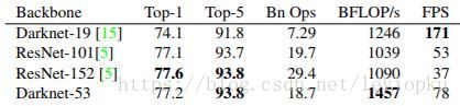
然后来看yolov3的输出,对于图1而言,更值得关注的是输出张量:

yolov3输出了3个不同尺度的feature map,如上图所示的y1, y2, y3。这也是v3论文中提到的为数不多的改进点:predictions across scales
这个借鉴了FPN(feature pyramid networks),采用多尺度来对不同size的目标进行检测,越精细的grid cell就可以检测出越精细的物体。
y1,y2和y3的深度都是255,边长的规律是13:26:52
对于COCO类别而言,有80个种类,所以每个box应该对每个种类都输出一个概率。
yolo v3设定的是每个网格单元预测3个box,所以每个box需要有(x, y, w, h, confidence)五个基本参数,然后还要有80个类别的概率。所以3*(5 + 80) = 255。这个255就是这么来的。(还记得yolo v1的输出张量吗? 7x7x30,只能识别20类物体,而且每个cell只能预测2个box)
v3用上采样的方法来实现这种多尺度的feature map,可以结合图1和图2右边来看,图1中concat连接的两个张量是具有一样尺度的(两处拼接分别是26x26尺度拼接和52x52尺度拼接,通过(2, 2)上采样来保证concat拼接的张量尺度相同)。作者并没有像SSD那样直接采用backbone中间层的处理结果作为feature map的输出,而是和后面网络层的上采样结果进行一个拼接之后的处理结果作为feature map。为什么这么做呢? 我感觉是有点玄学在里面,一方面避免和其他算法做法重合,另一方面这也许是试验之后并且结果证明更好的选择,再者有可能就是因为这么做比较节省模型size的。这点的数学原理不用去管,知道作者是这么做的就对了。
代码
utils.py
def compose(*funcs):
    """
    Compose arbitrarily many functions, evaluated left to right.

    Reference: https://mathieularose.com/function-composition-in-python/
    """
    # return lambda x: reduce(lambda v, f: f(v), funcs, x)
    if funcs:
        return reduce(lambda f, g: lambda *a, **kw: g(f(*a, **kw)), funcs)
    else:
        raise ValueError('Composition of empty sequence not supported.')
这个函数后面在神经网络中使用的非常之多,他的作用概括来说就是对funcs传来的函数列表,从左向右执行。也就是正序执行,如果是f(g(*a, **kw))就是倒序执行了。因为这个函数我认为很重要所以借鉴一下他人的详细讲解来看一下。
## 实现 F(x) = (x+1)*2
##
def compose2(f, g):
    return lambda x: f(g(x))   # lambda是匿名函数, 代表输入参数x, 输出f(g(x))
def double(x):
    return x * 2
def inc(x):
    return x + 1
inc_and_double = compose2(double, inc)(10)
print(inc_and_double)
结果:22
import functools
def dec(x):
    return x - 1;
def compose(*functions):
    return functools.reduce(lambda f,g: lambda x: f(g(x)),functions)
   # 1、functions代表输出参数有N函数, f第一次是取第N-1个函数,g是取第N个函数,
   # 2、step1 计算完结果作为第N-2个函数的输入,依次类推。当 f(g(x)) 改为g(f(x))时f,g从第0个函数开始取,相当于倒过来。
inc_double_and_dec = compose(dec,double,inc)(10)
print(inc_double_and_dec)
结果:21
然后是下一个方法:
def letterbox_image(image, size):
    """
    resize image with unchanged aspect ratio using padding
    """
    iw, ih = image.size
    w, h = size
    scale = min(w/iw, h/ih)
    nw = int(iw*scale)
    nh = int(ih*scale)

    image = image.resize((nw, nh), Image.BICUBIC)
    new_image = Image.new('RGB', size, (128, 128, 128))
    new_image.paste(image, ((w-nw)//2, (h-nh)//2))
    return new_image
这个方法的作用是是将输入的图像的尺寸改变为传入的size尺寸,其余部分填充颜色。
画个图可能更直观一些:

来看下一个函数:
def rand(a=0, b=1):
    return np.random.rand()*(b-a) + a
这个函数相比不用多说了,先引用一下:
np.random.rand(d0,d1,d2……dn)
注:使用方法与np.random.randn()函数相同
作用:
通过本函数可以返回一个或一组服从“0~1”均匀分布的随机样本值。随机样本取值范围是[0,1),不包括1。
应用:在深度学习的Dropout正则化方法中,可以用于生成dropout随机向量(dl),例如(keep_prob表示保留神经元的比例):dl = np.random.rand(al.shape[0],al.shape[1]) < keep_prob
结合一下这个函数的作用就是返回一个从a到b的均匀分布。
下一个函数:
def get_random_data(annotation_line,
                    input_shape,
                    random=True,
                    max_boxes=20,
                    jitter=.3,
                    hue=.1,
                    sat=1.5,
                    val=1.5,
                    proc_img=True):
    """
    random preprocessing for real-time data augmentation
    """
    line = annotation_line.split()
    image = Image.open(line[0])
    iw, ih = image.size
    h, w = input_shape
    box = np.array([np.array(list(map(int, box.split(',')))) for box in line[1:]])

    if not random:
        # resize image
        scale = min(w/iw, h/ih)
        nw = int(iw*scale)
        nh = int(ih*scale)
        dx = (w-nw)//2
        dy = (h-nh)//2
        image_data = 0
        if proc_img:
            image = image.resize((nw, nh), Image.BICUBIC)
            new_image = Image.new('RGB', (w, h), (128, 128, 128))
            new_image.paste(image, (dx, dy))
            image_data = np.array(new_image)/255.

        # correct boxes
        box_data = np.zeros((max_boxes, 5))
        if len(box) > 0:
            np.random.shuffle(box)
            if len(box) > max_boxes:
                box = box[:max_boxes]
            box[:, [0, 2]] = box[:, [0, 2]]*scale + dx
            box[:, [1, 3]] = box[:, [1, 3]]*scale + dy
            box_data[:len(box)] = box

        return image_data, box_data

    # resize image
    new_ar = w / h * rand(1 - jitter, 1 + jitter) / rand(1 - jitter, 1 + jitter)
    scale = rand(.25, 2)
    if new_ar < 1:
        nh = int(scale * h)
        nw = int(nh * new_ar)
    else:
        nw = int(scale * w)
        nh = int(nw / new_ar)
    image = image.resize((nw, nh), Image.BICUBIC)

    # place image
    dx = int(rand(0, w-nw))
    dy = int(rand(0, h-nh))
    new_image = Image.new('RGB', (w, h), (128, 128, 128))
    new_image.paste(image, (dx, dy))
    image = new_image

    # flip image or not
    flip = rand() < .5
    if flip:
        image = image.transpose(Image.FLIP_LEFT_RIGHT)

    # distort image
    hue = rand(-hue, hue)
    sat = rand(1, sat) if rand() < .5 else 1 / rand(1, sat)
    val = rand(1, val) if rand() < .5 else 1 / rand(1, val)
    x = rgb_to_hsv(np.array(image)/255.)
    x[..., 0] += hue
    x[..., 0][x[..., 0] > 1] -= 1
    x[..., 0][x[..., 0] < 0] += 1
    x[..., 1] *= sat
    x[..., 2] *= val
    x[x > 1] = 1
    x[x < 0] = 0
    # numpy array, 0 to 1
    image_data = hsv_to_rgb(x)

    # correct boxes
    box_data = np.zeros((max_boxes, 5))
    if len(box) > 0:
        np.random.shuffle(box)
        box[:, [0, 2]] = box[:, [0, 2]] * nw/iw + dx
        box[:, [1, 3]] = box[:, [1, 3]] * nh/ih + dy
        if flip:
            box[:, [0, 2]] = w - box[:, [2, 0]]
        box[:, 0:2][box[:, 0:2] < 0] = 0
        box[:, 2][box[:, 2] > w] = w
        box[:, 3][box[:, 3] > h] = h
        box_w = box[:, 2] - box[:, 0]
        box_h = box[:, 3] - box[:, 1]
        # discard invalid box
        box = box[np.logical_and(box_w > 1, box_h > 1)]
        if len(box) > max_boxes:
            box = box[:max_boxes]
        box_data[:len(box)] = box

    return image_data, box_data
这个函数有点长,我们一句一句来分析。
首先看传入的参数
annotation_line为传入的数据,是单条数据,以下面这条数据为例:
D:\yolotrain\VOCtrainval_11-May-2012\VOCdevkit\VOC2012\logistics_park_jpeg\2019_000015.jpg 1291,167,1329,254,0 1306,168,1321,184,2 1583,114,1920,346,1 1450,103,1506,155,1input_shape为输入图像的大小,在这里为(416,416)
line = annotation_line.split()
# 将数据用空格分开
image = Image.open(line[0])
# 第0个位置代表图片路径box = np.array([np.array(list(map(int, box.split(',')))) for box in line[1:]])
# box : [1294,167,1326,253,0 1303,164,1323,188,2 1590,128,1920,344,1 1446,103,1527,151,1]
# box.split(',') : [1294 167 1326 253 0]
# box :[
[1294 167 1326 253 0]
[1303 164 1323 188 2]
[1590 128 1920 344 1]
[1446 103 1527 151 1]
]if not random:
# 如果不随机。
# resize image
scale = min(w/iw, h/ih)
nw = int(iw*scale)
nh = int(ih*scale)
dx = (w-nw)//2
dy = (h-nh)//2
image_data = 0
if proc_img:
image = image.resize((nw, nh), Image.BICUBIC)
new_image = Image.new('RGB', (w, h), (128, 128, 128))
new_image.paste(image, (dx, dy))
image_data = np.array(new_image)/255.
# 这部分仿照letterbox_image的讲解
# correct boxes
box_data = np.zeros((max_boxes, 5))
# 创建一个 在这里是(20, 5)的0矩阵
if len(box) > 0:
# 上一步得到的box,如果数量大于0
np.random.shuffle(box)
# 对box进行打乱重排
if len(box) > max_boxes:
# 如果box数量大于20则只取前20个
box = box[:max_boxes]
box[:, [0, 2]] = box[:, [0, 2]]*scale + dx
box[:, [1, 3]] = box[:, [1, 3]]*scale + dy
# 这一步可以看下面的图
box_data[:len(box)] = box
return image_data, box_data
这样看来,这部分的作用其实就是将输入的图像进行整理,整理成要求的大小,如416*416,对box框也要根据图像尺寸的变化做相应的缩放和平移。
    # resize image
    new_ar = w / h * rand(1 - jitter, 1 + jitter) / rand(1 - jitter, 1 + jitter)
    scale = rand(.25, 2)
    if new_ar < 1:
        nh = int(scale * h)
        nw = int(nh * new_ar)
    else:
        nw = int(scale * w)
        nh = int(nw / new_ar)
    image = image.resize((nw, nh), Image.BICUBIC)
这部分代码主要是做数据增强,通过对图片尺度的随机改变增加训练集的数量。

    # flip image or not
    flip = rand() < .5
    if flip:
        image = image.transpose(Image.FLIP_LEFT_RIGHT)
    # 这部分代码对图像做随机的反转,也是数据增强的一种
# distort image
hue = rand(-hue, hue)
sat = rand(1, sat) if rand() < .5 else 1 / rand(1, sat)
val = rand(1, val) if rand() < .5 else 1 / rand(1, val)
x = rgb_to_hsv(np.array(image)/255.)
x[..., 0] += hue
x[..., 0][x[..., 0] > 1] -= 1
x[..., 0][x[..., 0] < 0] += 1
x[..., 1] *= sat
x[..., 2] *= val
x[x > 1] = 1
x[x < 0] = 0
# numpy array, 0 to 1
image_data = hsv_to_rgb(x)这一部分也是数据增强,是利用hsv色彩空间来做的,我们详细来看一下。
先大致了解一下hsv:
HSV颜色空间:HSV(hue,saturation,value)颜色空间的模型对应于圆柱坐标系中的一个圆锥形子集,圆锥的顶面对应于V=1. 它包含RGB模型中的R=1,G=1,B=1 三个面,所代表的颜色较亮。色彩H由绕V轴的旋转角给定。红色对应于 角度0° ,绿色对应于角度120°,蓝色对应于角度240°。在HSV颜色模型中,每一种颜色和它的补色相差180° 。 饱和度S取值从0到1,所以圆锥顶面的半径为1。HSV颜色模型所代表的颜色域是CIE色度图的一个子集,这个 模型中饱和度为百分之百的颜色,其纯度一般小于百分之百。在圆锥的顶点(即原点)处,V=0,H和S无定义, 代表黑色。圆锥的顶面中心处S=0,V=1,H无定义,代表白色。从该点到原点代表亮度渐暗的灰色,即具有不同 灰度的灰色。对于这些点,S=0,H的值无定义。可以说,HSV模型中的V轴对应于RGB颜色空间中的主对角线。 在圆锥顶面的圆周上的颜色,V=1,S=1,这种颜色是纯色。HSV模型对应于画家配色的方法。画家用改变色浓和 色深的方法从某种纯色获得不同色调的颜色,在一种纯色中加入白色以改变色浓,加入黑色以改变色深,同时 加入不同比例的白色,黑色即可获得各种不同的色调。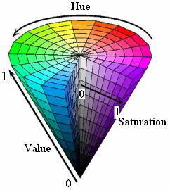
详细了解hsv与rgb关系的可以看这篇文章: RGB颜色空间、色调、饱和度、亮度、HSV颜色空间详解
了解了这些之后,上述代码其实就是在hsv第0维度(h),第一维度(s),第二维度(v)上分别做随机的改变,来随机图像增强。增加数据集。
    # correct boxes
    box_data = np.zeros((max_boxes, 5))
    if len(box) > 0:
        np.random.shuffle(box)
        box[:, [0, 2]] = box[:, [0, 2]] * nw/iw + dx
        box[:, [1, 3]] = box[:, [1, 3]] * nh/ih + dy
        if flip:
            box[:, [0, 2]] = w - box[:, [2, 0]]
        box[:, 0:2][box[:, 0:2] < 0] = 0
        box[:, 2][box[:, 2] > w] = w
        box[:, 3][box[:, 3] > h] = h
        box_w = box[:, 2] - box[:, 0]
        box_h = box[:, 3] - box[:, 1]
        # discard invalid box
        box = box[np.logical_and(box_w > 1, box_h > 1)]
        if len(box) > max_boxes:
            box = box[:max_boxes]
        box_data[:len(box)] = box

    return image_data, box_data
这些操作和之前不做random后边的操作相同,就是将box自适应为图像修改为制定大小后的大小。
这样utils这个脚本就分析完了。
convert.py
接下来我们来看看convert这个脚本吧,这个脚本虽然和模型训练预测关系不大,但是确是将官方权重转为h5文件的重要媒介,我们来看一看。
"""
Reads Darknet config and weights and creates Keras model with TF backend.

"""
顾名思义,就是将darknet配置转换为keras模型。
import argparse导入argparse模块,这个模块用于读取命令行
parser = argparse.ArgumentParser(description='Darknet To Keras Converter.')
parser.add_argument('config_path', help='Path to Darknet cfg file.')
parser.add_argument('weights_path', help='Path to Darknet weights file.')
parser.add_argument('output_path', help='Path to output Keras model file.')
parser.add_argument(
    '-p',
    '--plot_model',
    help='Plot generated Keras model and save as image.',
    action='store_true')
parser.add_argument(
    '-w',
    '--weights_only',
    help='Save as Keras weights file instead of model file.',
    action='store_true')
添加命令行参数,这里配合转化的命令来看更加清晰。
下面来看另一个函数:
def unique_config_sections(config_file):
    """
    Convert all config sections to have unique names.

    Adds unique suffixes to config sections for compability with configparser.
    """
    section_counters = defaultdict(int)
    # 创一个默认键值为int的字典
    output_stream = io.StringIO()
    # 初始化io操作
    with open(config_file) as fin:
        for line in fin:
            if line.startswith('['):
                section = line.strip().strip('[]')
                # 取出[]中的值
                _section = section + '_' + str(section_counters[section])
                section_counters[section] += 1
                line = line.replace(section, _section)
            output_stream.write(line)
    output_stream.seek(0)
    return output_stream
此函数的作用是按照行来读取config文件,对[convolutional]这样的行,会将[]中的内容取出并带上该标签的值,例如:
[convolutional]将会变成[convolutional_2]。
下面来看这个脚本的主要的函数:
def _main(args):
    # 配置文件路径
    config_path = os.path.expanduser(args.config_path)
    # darknet 权重文件路径
    weights_path = os.path.expanduser(args.weights_path)
    # 断言不是.cfg就退出
    assert config_path.endswith('.cfg'), '{} is not a .cfg file'.format(
        config_path)
    # 断言不是weights结尾就退出
    assert weights_path.endswith(
        '.weights'), '{} is not a .weights file'.format(weights_path)
    # 设置输出路径
    output_path = os.path.expanduser(args.output_path)
    # 断言不是h5结尾就退出
    assert output_path.endswith(
        '.h5'), 'output path {} is not a .h5 file'.format(output_path)
    # print(os.path.splitext('yolo.cfg')) ==》('yolo', '.cfg')
    output_root = os.path.splitext(output_path)[0]

    # Load weights and config.
    print('Loading weights.')
    # 权重文件的版本和头信息
    weights_file = open(weights_path, 'rb')
    major, minor, revision = np.ndarray(shape=(3, ), dtype='int32', buffer=weights_file.read(12))
    if (major*10+minor) >= 2 and major < 1000 and minor < 1000:
        seen = np.ndarray(shape=(1,), dtype='int64', buffer=weights_file.read(8))
    else:
        seen = np.ndarray(shape=(1,), dtype='int32', buffer=weights_file.read(4))
    print('Weights Header: ', major, minor, revision, seen)

    print('Parsing Darknet config.')
    # 获取修改后的config文件
    unique_config_file = unique_config_sections(config_path)
    cfg_parser = configparser.ConfigParser()
    cfg_parser.read_file(unique_config_file)

    print('Creating Keras model.')
    input_layer = Input(shape=(None, None, 3))
    prev_layer = input_layer
    all_layers = []
    # 设置权重衰减项
    weight_decay = float(cfg_parser['net_0']['decay']) if 'net_0' in cfg_parser.sections() else 5e-4
    count = 0
    out_index = []
    for section in cfg_parser.sections():
        print('Parsing section {}'.format(section))
        if section.startswith('convolutional'):
            filters = int(cfg_parser[section]['filters'])
            size = int(cfg_parser[section]['size'])
            stride = int(cfg_parser[section]['stride'])
            pad = int(cfg_parser[section]['pad'])
            activation = cfg_parser[section]['activation']
            batch_normalize = 'batch_normalize' in cfg_parser[section]

            padding = 'same' if pad == 1 and stride == 1 else 'valid'

            # Setting weights.
            # Darknet serializes convolutional weights as:
            # [bias/beta, [gamma, mean, variance], conv_weights]
            # 例如
            # input_layer = Input(shape=(416, 416, 3))
            # prev_layer_shape = K.int_shape(input_layer)
            # print(prev_layer_shape) ==》(None, 416, 416, 3)
            prev_layer_shape = K.int_shape(prev_layer)

            # prev_layer_shape[-1] ==》 3
            weights_shape = (size, size, prev_layer_shape[-1], filters)
            darknet_w_shape = (filters, weights_shape[2], size, size)
            # size * size * 3 * filters
            # np.product(x):求n维数组所有元素的乘积
            weights_size = np.product(weights_shape)

            print('conv2d', 'bn' if batch_normalize else '  ', activation, weights_shape)
            # 读取卷积层 bias数据
            conv_bias = np.ndarray(
                shape=(filters, ),
                dtype='float32',
                buffer=weights_file.read(filters * 4))
            count += filters
            # 如果有bn层
            if batch_normalize:
                # 读取bn层的权重,有三层
                bn_weights = np.ndarray(
                    shape=(3, filters),
                    dtype='float32',
                    buffer=weights_file.read(filters * 12))
                count += 3 * filters

                bn_weight_list = [
                    bn_weights[0],  # scale gamma
                    conv_bias,  # shift beta
                    bn_weights[1],  # running mean
                    bn_weights[2]  # running var
                ]
            # 读取卷基层的 w数据
            conv_weights = np.ndarray(
                shape=darknet_w_shape,
                dtype='float32',
                buffer=weights_file.read(weights_size * 4))
            count += weights_size

            # DarkNet conv_weights are serialized Caffe-style:
            # (out_dim, in_dim, height, width)
            # We would like to set these to Tensorflow order:
            # (height, width, in_dim, out_dim)
            # 维度转换从caffe转为tensorflow
            conv_weights = np.transpose(conv_weights, [2, 3, 1, 0])
            conv_weights = [conv_weights] if batch_normalize else [conv_weights, conv_bias]

            # Handle activation.
            # 判断激活函数是不是leaky
            act_fn = None
            if activation == 'leaky':
                pass  # Add advanced activation later.
            elif activation != 'linear':
                raise ValueError(
                    'Unknown activation function `{}` in section {}'.format(
                        activation, section))

            # Create Conv2D layer
            if stride > 1:
                # 如果步长大于1,则增加padding
                # Darknet uses left and top padding instead of 'same' mode
                prev_layer = ZeroPadding2D(((1, 0), (1, 0)))(prev_layer)
            # 卷基层
            conv_layer = (
                            Conv2D(filters,
                                   (size, size),
                                   strides=(stride, stride),
                                   kernel_regularizer=l2(weight_decay),
                                   use_bias=not batch_normalize,
                                   weights=conv_weights,
                                   activation=act_fn,
                                   padding=padding)
                         )(prev_layer)

            if batch_normalize:
                # 如果有bn如要加上bn
                conv_layer = (BatchNormalization(weights=bn_weight_list))(conv_layer)
            prev_layer = conv_layer

            if activation == 'linear':
                all_layers.append(prev_layer)
            elif activation == 'leaky':
                act_layer = LeakyReLU(alpha=0.1)(prev_layer)
                prev_layer = act_layer
                # 将该层添加到总的层级里
                all_layers.append(act_layer)

        elif section.startswith('route'):
            # route层 例如
            # [route]
            # layers = -1, 61
            # [route]
            # layers = -4
            ids = [int(i) for i in cfg_parser[section]['layers'].split(',')]
            # 取出该层
            layers = [all_layers[i] for i in ids]
            if len(layers) > 1:
                # 如果是层数大于1的情况,将两层拼接起来,并添加到总层级
                print('Concatenating route layers:', layers)
                concatenate_layer = Concatenate()(layers)
                all_layers.append(concatenate_layer)
                prev_layer = concatenate_layer
            else:
                # 如果只有一层就是直接把这层添加进去
                skip_layer = layers[0]  # only one layer to route
                all_layers.append(skip_layer)
                prev_layer = skip_layer

        elif section.startswith('maxpool'):
            # 最大池化层
            size = int(cfg_parser[section]['size'])
            stride = int(cfg_parser[section]['stride'])
            all_layers.append(
                MaxPooling2D(
                    pool_size=(size, size),
                    strides=(stride, stride),
                    padding='same')(prev_layer))
            prev_layer = all_layers[-1]

        elif section.startswith('shortcut'):
            # [shortcut]
            # from=-3
            # activation = linear
            # 找到上边的某一层将结果相加
            index = int(cfg_parser[section]['from'])
            activation = cfg_parser[section]['activation']
            assert activation == 'linear', 'Only linear activation supported.'
            all_layers.append(Add()([all_layers[index], prev_layer]))
            prev_layer = all_layers[-1]

        elif section.startswith('upsample'):
            # 上采样
            stride = int(cfg_parser[section]['stride'])
            # 只支持两倍上采样
            assert stride == 2, 'Only stride=2 supported.'
            all_layers.append(UpSampling2D(stride)(prev_layer))
            prev_layer = all_layers[-1]

        elif section.startswith('yolo'):
            # yolo层 例如
            # [yolo]
            # mask = 6, 7, 8
            # anchors = 10, 13, 16, 30, 33, 23, 30, 61, 62, 45, 59, 119, 116, 90, 156, 198, 373, 326
            # classes = 8
            # num = 9
            # jitter = .3
            # ignore_thresh = .5
            # truth_thresh = 1
            # random = 1
            out_index.append(len(all_layers)-1)
            # 添加none
            all_layers.append(None)
            prev_layer = all_layers[-1]

        elif section.startswith('net'):
            pass

        else:
            raise ValueError(
                'Unsupported section header type: {}'.format(section))

    # Create and save model.
    if len(out_index) == 0:
        # 如果没有yolo层,则用最后一层作为yolo层
        out_index.append(len(all_layers)-1)
    # 初始化模型
    model = Model(inputs=input_layer, outputs=[all_layers[i] for i in out_index])
    print(model.summary())
    if args.weights_only:
        model.save_weights('{}'.format(output_path))
        print('Saved Keras weights to {}'.format(output_path))
    else:
        model.save('{}'.format(output_path))
        print('Saved Keras model to {}'.format(output_path))

    # Check to see if all weights have been read.
    remaining_weights = len(weights_file.read()) / 4
    weights_file.close()
    print('Read {} of {} from Darknet weights.'.format(count, count +
                                                       remaining_weights))
    if remaining_weights > 0:
        print('Warning: {} unused weights'.format(remaining_weights))

    if args.plot_model:
        plot(model, to_file='{}.png'.format(output_root), show_shapes=True)
        print('Saved model plot to {}.png'.format(output_root))
这个函数的功能已经在代码中间写了注释,主要就是根据cfg来制作模型。
voc_annotation.py
接下来看下一个脚本,voc_annotation.py,和另一个基于coco数据集的coco_annotation.py,这两个脚本的原理相同,这里只说前者。
sets = [('2007', 'train'), ('2007', 'val'), ('2007', 'test')]

classes = ["aeroplane", "bicycle", "bird", "boat", "bottle",
           "bus", "car", "cat", "chair", "cow",
           "diningtable", "dog", "horse", "motorbike", "person",
           "pottedplant", "sheep", "sofa", "train", "tvmonitor"]
sets的意思就是三种数据集,训练集,验证集,测试集
classes是你训练集中要训练的类别。
def convert_annotation(year, image_id, list_file):
    in_file = open('VOCdevkit/VOC%s/Annotations/%s.xml' % (year, image_id))
    tree = ET.parse(in_file)
    root = tree.getroot()

    for obj in root.iter('object'):
        difficult = obj.find('difficult').text
        cls = obj.find('name').text
        if cls not in classes or int(difficult) == 1:
            continue
        cls_id = classes.index(cls)
        xmlbox = obj.find('bndbox')
        b = (int(xmlbox.find('xmin').text),
             int(xmlbox.find('ymin').text),
             int(xmlbox.find('xmax').text),
             int(xmlbox.find('ymax').text))
        list_file.write(" " + ",".join([str(a) for a in b]) + ',' + str(cls_id))
这里说一下,我们训练的时候,要自己制作训练集,如何从头开始训练自己的yolo会在后面讲,这里我们简单说一下,我们会使用labelimage的一个软件。将我们的训练图片手动圈出物体并设置类别,保存之后会生成一个对应的xml文件,文件中保存着我们圈出物体框的位置大小还有类别。
上边这个函数的作用就是读取xml文件,将我们标注的方框找到坐标值和类别值写入到一个文件中去。
for year, image_set in sets:
    image_ids = open('VOCdevkit/VOC%s/ImageSets/Main/%s.txt' % (year, image_set)).read().strip().split()
    list_file = open('%s_%s.txt' % (year, image_set), 'w')
    for image_id in image_ids:
        list_file.write('%s/VOCdevkit/VOC%s/JPEGImages/%s.jpg' % (wd, year, image_id))
        convert_annotation(year, image_id, list_file)
        list_file.write('\n')
    list_file.close()
这个函数对三种不同种类的数据集分别做上述函数的操作。
kmeans.py
下面我们来看kmeans.py这个脚本。里面最主要的部分是一个class:
class YOLO_Kmeans:

    def __init__(self, cluster_number, filename):
        self.cluster_number = cluster_number
        self.filename = "2012_train.txt"

    def iou(self, boxes, clusters):  # 1 box -> k clusters
        n = boxes.shape[0]
        k = self.cluster_number

        box_area = boxes[:, 0] * boxes[:, 1]
        box_area = box_area.repeat(k)
        box_area = np.reshape(box_area, (n, k))

        cluster_area = clusters[:, 0] * clusters[:, 1]
        cluster_area = np.tile(cluster_area, [1, n])
        cluster_area = np.reshape(cluster_area, (n, k))

        box_w_matrix = np.reshape(boxes[:, 0].repeat(k), (n, k))
        cluster_w_matrix = np.reshape(np.tile(clusters[:, 0], (1, n)), (n, k))
        min_w_matrix = np.minimum(cluster_w_matrix, box_w_matrix)

        box_h_matrix = np.reshape(boxes[:, 1].repeat(k), (n, k))
        cluster_h_matrix = np.reshape(np.tile(clusters[:, 1], (1, n)), (n, k))
        min_h_matrix = np.minimum(cluster_h_matrix, box_h_matrix)
        inter_area = np.multiply(min_w_matrix, min_h_matrix)

        result = inter_area / (box_area + cluster_area - inter_area)
        return result

    def avg_iou(self, boxes, clusters):
        accuracy = np.mean([np.max(self.iou(boxes, clusters), axis=1)])
        return accuracy

    def kmeans(self, boxes, k, dist=np.median):
        box_number = boxes.shape[0]
        distances = np.empty((box_number, k))
        last_nearest = np.zeros((box_number,))
        np.random.seed()
        # init k clusters
        clusters = boxes[np.random.choice(box_number, k, replace=False)]
        while True:

            distances = 1 - self.iou(boxes, clusters)

            current_nearest = np.argmin(distances, axis=1)
            if (last_nearest == current_nearest).all():
                break  # clusters won't change
            for cluster in range(k):
                clusters[cluster] = dist(  # update clusters
                    boxes[current_nearest == cluster], axis=0)

            last_nearest = current_nearest

        return clusters

    def result2txt(self, data):
        f = open("yolo_anchors.txt", 'w')
        row = np.shape(data)[0]
        for i in range(row):
            if i == 0:
                x_y = "%d,%d" % (data[i][0], data[i][1])
            else:
                x_y = ", %d,%d" % (data[i][0], data[i][1])
            f.write(x_y)
        f.close()

    def txt2boxes(self):
        f = open(self.filename, 'r')
        dataSet = []
        for line in f:
            infos = line.split(" ")
            length = len(infos)
            for i in range(1, length):
                width = int(infos[i].split(",")[2]) - int(infos[i].split(",")[0])
                height = int(infos[i].split(",")[3]) - int(infos[i].split(",")[1])
                dataSet.append([width, height])
        result = np.array(dataSet)
        f.close()
        return result

    def txt2clusters(self):
        all_boxes = self.txt2boxes()
        result = self.kmeans(all_boxes, k=self.cluster_number)
        result = result[np.lexsort(result.T[0, None])]
        self.result2txt(result)
        print("K anchors:\n {}".format(result))
        print("Accuracy: {:.2f}%".format(self.avg_iou(all_boxes, result) * 100))
我们详细剖析一下这个class。
我们先看主函数是如何调用的:
if __name__ == "__main__":
    cluster_number = 9
    filename = "2012_train.txt"
    kmeans = YOLO_Kmeans(cluster_number, filename)
    kmeans.txt2clusters()
D:\yolotrain\VOCtrainval_11-May-2012\VOCdevkit\VOC2012\logistics_park_jpeg\2019_000016.jpg 1296,164,1324,255,0 1307,168,1324,188,2 1590,135,1920,342,1 1446,104,1504,158,1
D:\yolotrain\VOCtrainval_11-May-2012\VOCdevkit\VOC2012\logistics_park_jpeg\2019_000017.jpg 1294,167,1326,253,0 1303,164,1323,188,2 1590,128,1920,344,1 1446,103,1527,151,1train.txt可以是长这个样子的。
我们从这个函数入手:
    def txt2boxes(self):
        f = open(self.filename, 'r')
        # 读取train.txt
        dataSet = []
        for line in f:
            infos = line.split(" ")
            length = len(infos)
            # 剔除掉第0个位置的路径信息,剩下的就是方框的位置信息
            for i in range(1, length):
                # 获取宽度
                width = int(infos[i].split(",")[2]) - int(infos[i].split(",")[0])
                # 获取高度
                height = int(infos[i].split(",")[3]) - int(infos[i].split(",")[1])
                # 放入dataset中
                dataSet.append([width, height])
        result = np.array(dataSet)
        f.close()
        return result
然后看这个函数:
    def iou(self, boxes, clusters):  # 1 box -> k clusters
        # boxes为所有的框 boxes[weight,height]
        n = boxes.shape[0]
        k = self.cluster_number

        box_area = boxes[:, 0] * boxes[:, 1]

        # 重复并且展平.
        # boxes = [[5, 10],[6, 8],[4, 7], ... Xn]
        # k = 9 处理后变为 [50, 50, ... X9, 48, 48, ... X9, 28, 28, ... X9, ... Xn]
        box_area = box_area.repeat(k)
        # reshape变为[
        #       [50, 50, ... X9],
        #       [48, 48, ... X9],
        #       [28, 28, ... X9],
        #            ... Xn
        # ]
        box_area = np.reshape(box_area, (n, k))

        # 这里也是重复操作但是处理方式不同
        # clusters长度为9
        cluster_area = clusters[:, 0] * clusters[:, 1]
        # clusters长度为3, clusters = [[5, 10],[6, 8],[4, 7]... X9]
        # cluster_area = [50, 48, 28, ... X9]
        # tile后为 [
        #            [50, 48, 28, ... X9, 50, 48, 28, ... X9, 50, 48, 28, ... X9 ... Xn]
        # ]
        cluster_area = np.tile(cluster_area, [1, n])
        # reshape后变为:
        # [
        #      [50, 48, 28, ... X9],
        #            ... Xn
        #      [50, 48, 28, ... X9]
        # ]
        cluster_area = np.reshape(cluster_area, (n, k))

        #这个操作同上,样例可以参照下边的手动分析
        box_w_matrix = np.reshape(boxes[:, 0].repeat(k), (n, k))
        cluster_w_matrix = np.reshape(np.tile(clusters[:, 0], (1, n)), (n, k))
        min_w_matrix = np.minimum(cluster_w_matrix, box_w_matrix)

        box_h_matrix = np.reshape(boxes[:, 1].repeat(k), (n, k))
        cluster_h_matrix = np.reshape(np.tile(clusters[:, 1], (1, n)), (n, k))
        min_h_matrix = np.minimum(cluster_h_matrix, box_h_matrix)
        inter_area = np.multiply(min_w_matrix, min_h_matrix)
        # 交并比
        result = inter_area / (box_area + cluster_area - inter_area)
        return result

这个函数是计算iou也就是交并比的一个函数。
下面看kmean函数,这个是kmean算法的核心思想:
    def kmeans(self, boxes, k, dist=np.median):
        # boxes为全部的框的宽度和高度
        # 获取数量
        box_number = boxes.shape[0]
        distances = np.empty((box_number, k))
        last_nearest = np.zeros((box_number,))
        np.random.seed()
        # init k clusters
        # 先随机选择了9条
        # clusters ==》 (9, 9)
        clusters = boxes[np.random.choice(box_number, k, replace=False)]
        while True:

            # 算法中有说明使用 iou来衡量聚类的指标,而不使用欧式距离,避免因框体大小不同产生误差
            distances = 1 - self.iou(boxes, clusters)

            # distances ==》 (20, 9)
            current_nearest = np.argmin(distances, axis=1)
            # current_nearest ==》 (20, 1)
            if (last_nearest == current_nearest).all():
                # clusters不在变化了就退出
                break  # clusters won't change
            for cluster in range(k):
                # 重新选择9个数据作为cluster
                clusters[cluster] = dist(  # update clusters
                    boxes[current_nearest == cluster], axis=0)

            last_nearest = current_nearest

        return clusters
这个函数意思就是,每次使用9个box数据,与所有的boxes数据进行iou的计算,每次计算出一个(20,9)的distance,对每一行取最小值就是获取到了20个框框最小的iou数据,然后使用这些好的数据再次放入总的boxes数据中寻找最优的iou的box。
这个方法说是k均值,但是琢磨了很长时间还是觉得和传统k均值差距很大,应该有自己的算法思想。我的理解就是第一次随机取出9个boxes 和 总得的boxes假设这里总共有100个boxes,计算出一个(100, 9)的iou数据,这个数据就是100个box中每个box的9类iou,对每一个box取最小的iou,和全局最优iou做对比,如果没有发生变化了就退出,否则继续,从100个box的最优iou中重新选择9个box作为新的clusters,重新放入100个boxes中进行寻找,依次往复。
    def result2txt(self, data):
        f = open("yolo_anchors.txt", 'w')
        row = np.shape(data)[0]
        for i in range(row):
            if i == 0:
                x_y = "%d,%d" % (data[i][0], data[i][1])
            else:
                x_y = ", %d,%d" % (data[i][0], data[i][1])
            f.write(x_y)
        f.close()
这个函数的作用是将前边算好的框写入到文件中去。
    def txt2clusters(self):
        # 收集所有的框
        all_boxes = self.txt2boxes()
        # 对框做聚类,得到9类
        result = self.kmeans(all_boxes, k=self.cluster_number)
        # result ==> (9, 2), 重新排序
        result = result[np.lexsort(result.T[0, None])]
        # 写入anchors文件中
        self.result2txt(result)
        print("K anchors:\n {}".format(result))
        print("Accuracy: {:.2f}%".format(self.avg_iou(all_boxes, result) * 100))
这个函数是类的控制函数,一套流水线,看一看注释来理解。
model.py
接下来我们就从数据集的准备过程进入到yolo模型的设计过程,我们来看看yolo模型的脚本。
首先整个yolo-keras中最重要也是最难理解的脚本就是model.py我们接下来啃一啃这块骨头。
@wraps(Conv2D)
def DarknetConv2D(*args, **kwargs):
    """
    Wrapper to set Darknet parameters for Convolution2D.
    """
    darknet_conv_kwargs = {'kernel_regularizer': l2(5e-4)}
    darknet_conv_kwargs['padding'] = 'valid' if kwargs.get('strides') == (2, 2) else 'same'
    darknet_conv_kwargs.update(kwargs)
    return Conv2D(*args, **darknet_conv_kwargs)
这个函数就是定义一个卷基层,这个函数是一个基础单元,用于后边调用的。接收传过来的 *args list类型参数,和**kwargs dict类型参数,用于设置卷基层的各项参数和更新各项参数。
def DarknetConv2D_BN_Leaky(*args, **kwargs):
    """
    Darknet Convolution2D followed by BatchNormalization and LeakyReLU.
    """
    no_bias_kwargs = {'use_bias': False}
    no_bias_kwargs.update(kwargs)
    return compose(
        DarknetConv2D(*args, **no_bias_kwargs),
        BatchNormalization(),
        LeakyReLU(alpha=0.1))
这同样是一个基础单元,是一个增加了BN层和LeakyRelu层的卷基层。compose函数在utils脚本中已经介绍过,这里是从上到下依次执行。同样使用*args, **kwargs动态更新设置网络层的参数。
def resblock_body(x, num_filters, num_blocks):
    """
    A series of resblocks starting with a downsampling Convolution2D
    """
    # Darknet uses left and top padding instead of 'same' mode
    x = ZeroPadding2D(((1, 0), (1, 0)))(x)
    x = DarknetConv2D_BN_Leaky(num_filters, (3, 3), strides=(2, 2))(x)
    for i in range(num_blocks):
        y = compose(
                DarknetConv2D_BN_Leaky(num_filters // 2, (1, 1)),
                DarknetConv2D_BN_Leaky(num_filters, (3, 3)))(x)
        x = Add()([x, y])
    return x
这个模块就是resblock模块,可以对应下图进行理解。
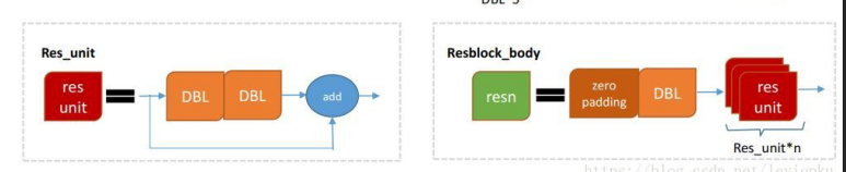
先接一个0的padding层,然后接一个bn + rulu + 卷积层,然后进入res_unit单元,循环后和上一层卷积层相加。
def darknet_body(x):

    """
    Darknent body having 52 Convolution2D layers
    """

    x = DarknetConv2D_BN_Leaky(32, (3, 3))(x)
    x = resblock_body(x, 64, 1)
    x = resblock_body(x, 128, 2)
    x = resblock_body(x, 256, 8)
    x = resblock_body(x, 512, 8)
    x = resblock_body(x, 1024, 4)
    return x
这个就是darknet网络的结构代码表示。再看看这一张图。就是这张图的前半部分。
def make_last_layers(x, num_filters, out_filters):
    """
    6 Conv2D_BN_Leaky layers followed by a Conv2D_linear layer
    """
    x = compose(
            DarknetConv2D_BN_Leaky(num_filters, (1, 1)),
            DarknetConv2D_BN_Leaky(num_filters*2, (3, 3)),
            DarknetConv2D_BN_Leaky(num_filters, (1, 1)),
            DarknetConv2D_BN_Leaky(num_filters*2, (3, 3)),
            DarknetConv2D_BN_Leaky(num_filters, (1, 1)))(x)
    y = compose(
            DarknetConv2D_BN_Leaky(num_filters*2, (3, 3)),
            DarknetConv2D(out_filters, (1, 1)))(x)
    return x, y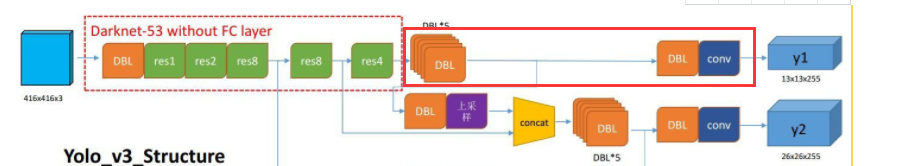
结合图来看就是红色框框的部分。
def yolo_body(inputs, num_anchors, num_classes):
    """
    Create YOLO_V3 model CNN body in Keras.
    """
    darknet = Model(inputs, darknet_body(inputs))
    x, y1 = make_last_layers(darknet.output, 512, num_anchors*(num_classes+5))

    x = compose(
            DarknetConv2D_BN_Leaky(256, (1, 1)),
            UpSampling2D(2))(x)
    x = Concatenate()([x, darknet.layers[152].output])
    x, y2 = make_last_layers(x, 256, num_anchors*(num_classes+5))

    x = compose(
            DarknetConv2D_BN_Leaky(128, (1, 1)),
            UpSampling2D(2))(x)
    x = Concatenate()([x, darknet.layers[92].output])
    x, y3 = make_last_layers(x, 128, num_anchors*(num_classes+5))

    return Model(inputs, [y1, y2, y3])
首先创建darknet的模型结构。
然后使用darknet的输出作为yolo后边自定义的输入,进入上图红框部分,x为经过5个卷积层后。
对x进行卷积 + bn + relu操作,后执行2倍的上采样,使图像大小和darknetmodel中的152层大小相同。

然后和152层进行叠加记为x,x继续进行make_last_layers,输出继续做卷积 + bn + rulu,同样进行一个上采样后,与darknet的第92层进行叠加,叠加后再次进行make_last_layers,得到三种输出,y1, y2, y3。
def tiny_yolo_body(inputs, num_anchors, num_classes):
    """
    Create Tiny YOLO_v3 model CNN body in keras.
    """
    x1 = compose(
            DarknetConv2D_BN_Leaky(16, (3, 3)),
            MaxPooling2D(pool_size=(2, 2), strides=(2, 2), padding='same'),
            DarknetConv2D_BN_Leaky(32, (3, 3)),
            MaxPooling2D(pool_size=(2, 2), strides=(2, 2), padding='same'),
            DarknetConv2D_BN_Leaky(64, (3, 3)),
            MaxPooling2D(pool_size=(2, 2), strides=(2, 2), padding='same'),
            DarknetConv2D_BN_Leaky(128, (3, 3)),
            MaxPooling2D(pool_size=(2, 2), strides=(2, 2), padding='same'),
            DarknetConv2D_BN_Leaky(256, (3, 3)))(inputs)
    x2 = compose(
            MaxPooling2D(pool_size=(2, 2), strides=(2, 2), padding='same'),
            DarknetConv2D_BN_Leaky(512, (3, 3)),
            MaxPooling2D(pool_size=(2, 2), strides=(1, 1), padding='same'),
            DarknetConv2D_BN_Leaky(1024, (3, 3)),
            DarknetConv2D_BN_Leaky(256, (1, 1)))(x1)
    y1 = compose(
            DarknetConv2D_BN_Leaky(512, (3, 3)),
            DarknetConv2D(num_anchors*(num_classes+5), (1, 1)))(x2)

    x2 = compose(
            DarknetConv2D_BN_Leaky(128, (1, 1)),
            UpSampling2D(2))(x2)
    y2 = compose(
            Concatenate(),
            DarknetConv2D_BN_Leaky(256, (3, 3)),
            DarknetConv2D(num_anchors*(num_classes+5), (1, 1)))([x2, x1])

    return Model(inputs, [y1, y2])
这个是tinyyolo的网络结构,还保留池化层,只有一次上采样。
下面看一个函数:
def yolo_head(feats, anchors, num_classes, input_shape, calc_loss=False):
    """
    Convert final layer features to bounding box parameters.
    """
    # 获取框的个数
    num_anchors = len(anchors)
    # Reshape to batch, height, width, num_anchors, box_params.
    anchors_tensor = K.reshape(K.constant(anchors), [1, 1, 1, num_anchors, 2])

    # height, width
    grid_shape = K.shape(feats)[1:3]
    grid_y = K.tile(K.reshape(K.arange(0, stop=grid_shape[0]), [-1, 1, 1, 1]), [1, grid_shape[1], 1, 1])
    grid_x = K.tile(K.reshape(K.arange(0, stop=grid_shape[1]), [1, -1, 1, 1]), [grid_shape[0], 1, 1, 1])
    grid = K.concatenate([grid_x, grid_y])
    grid = K.cast(grid, K.dtype(feats))

    feats = K.reshape(feats, [-1, grid_shape[0], grid_shape[1], num_anchors, num_classes + 5])

    # Adjust predictions to each spatial grid point and anchor size.
    box_xy = (K.sigmoid(feats[..., :2]) + grid) / K.cast(grid_shape[::-1], K.dtype(feats))
    box_wh = K.exp(feats[..., 2:4]) * anchors_tensor / K.cast(input_shape[::-1], K.dtype(feats))
    box_confidence = K.sigmoid(feats[..., 4:5])
    box_class_probs = K.sigmoid(feats[..., 5:])

    if calc_loss:
        return grid, feats, box_xy, box_wh
    return box_xy, box_wh, box_confidence, box_class_probs
这个函数我觉得很不好理解,所以先把关注点放在前面几行对网格的操作。这个函数篇幅会有一点长,做好心理准备。
feats为yolo模型输出矩阵,第一维是batch_size,第二维和第三维是输出特征的大小,这里有三种,13*13,26*26,52*52,第四维是255,结合理论部分分析,这里不再赘述。
grid_shape取到这些大小,假设取得的值为13 * 13.
    grid_shape = K.shape(feats)[1:3]
    grid_y = K.tile(K.reshape(K.arange(0, stop=grid_shape[0]), [-1, 1, 1, 1]), [1, grid_shape[1], 1, 1])
    grid_x = K.tile(K.reshape(K.arange(0, stop=grid_shape[1]), [1, -1, 1, 1]), [grid_shape[0], 1, 1, 1])
    grid = K.concatenate([grid_x, grid_y])
    grid = K.cast(grid, K.dtype(feats))
这段代码的作用是制作网格,可以参考理论知识,yolo是对图像进行网格的划分的。
可以看下面的示例程序。
    a = K.reshape(K.arange(0, stop=13), [-1, 1, 1, 1])
    print(a.eval())
    print('-------------------------------------')
输出:
[[[[ 0]]]


 [[[ 1]]]


 [[[ 2]]]


 [[[ 3]]]


 [[[ 4]]]


 [[[ 5]]]


 [[[ 6]]]


 [[[ 7]]]


 [[[ 8]]]


 [[[ 9]]]


 [[[10]]]


 [[[11]]]


 [[[12]]]]
-------------------------------------
b = K.tile(a, [1, 13, 1, 1])
print(b.eval())
print('-------------------------------------')输出:
[[[[ 0]]

  [[ 0]]

  [[ 0]]

  [[ 0]]

  [[ 0]]

  [[ 0]]

  [[ 0]]

  [[ 0]]

  [[ 0]]

  [[ 0]]

  [[ 0]]

  [[ 0]]

  [[ 0]]]


 [[[ 1]]

  [[ 1]]

  [[ 1]]

  [[ 1]]

  [[ 1]]

  [[ 1]]

  [[ 1]]

  [[ 1]]

  [[ 1]]

  [[ 1]]

  [[ 1]]

  [[ 1]]

  [[ 1]]]


 [[[ 2]]

  [[ 2]]

  [[ 2]]

  [[ 2]]

  [[ 2]]

  [[ 2]]

  [[ 2]]

  [[ 2]]

  [[ 2]]

  [[ 2]]

  [[ 2]]

  [[ 2]]

  [[ 2]]]


 [[[ 3]]

  [[ 3]]

  [[ 3]]

  [[ 3]]

  [[ 3]]

  [[ 3]]

  [[ 3]]

  [[ 3]]

  [[ 3]]

  [[ 3]]

  [[ 3]]

  [[ 3]]

  [[ 3]]]


 [[[ 4]]

  [[ 4]]

  [[ 4]]

  [[ 4]]

  [[ 4]]

  [[ 4]]

  [[ 4]]

  [[ 4]]

  [[ 4]]

  [[ 4]]

  [[ 4]]

  [[ 4]]

  [[ 4]]]


 [[[ 5]]

  [[ 5]]

  [[ 5]]

  [[ 5]]

  [[ 5]]

  [[ 5]]

  [[ 5]]

  [[ 5]]

  [[ 5]]

  [[ 5]]

  [[ 5]]

  [[ 5]]

  [[ 5]]]


 [[[ 6]]

  [[ 6]]

  [[ 6]]

  [[ 6]]

  [[ 6]]

  [[ 6]]

  [[ 6]]

  [[ 6]]

  [[ 6]]

  [[ 6]]

  [[ 6]]

  [[ 6]]

  [[ 6]]]


 [[[ 7]]

  [[ 7]]

  [[ 7]]

  [[ 7]]

  [[ 7]]

  [[ 7]]

  [[ 7]]

  [[ 7]]

  [[ 7]]

  [[ 7]]

  [[ 7]]

  [[ 7]]

  [[ 7]]]


 [[[ 8]]

  [[ 8]]

  [[ 8]]

  [[ 8]]

  [[ 8]]

  [[ 8]]

  [[ 8]]

  [[ 8]]

  [[ 8]]

  [[ 8]]

  [[ 8]]

  [[ 8]]

  [[ 8]]]


 [[[ 9]]

  [[ 9]]

  [[ 9]]

  [[ 9]]

  [[ 9]]

  [[ 9]]

  [[ 9]]

  [[ 9]]

  [[ 9]]

  [[ 9]]

  [[ 9]]

  [[ 9]]

  [[ 9]]]


 [[[10]]

  [[10]]

  [[10]]

  [[10]]

  [[10]]

  [[10]]

  [[10]]

  [[10]]

  [[10]]

  [[10]]

  [[10]]

  [[10]]

  [[10]]]


 [[[11]]

  [[11]]

  [[11]]

  [[11]]

  [[11]]

  [[11]]

  [[11]]

  [[11]]

  [[11]]

  [[11]]

  [[11]]

  [[11]]

  [[11]]]


 [[[12]]

  [[12]]

  [[12]]

  [[12]]

  [[12]]

  [[12]]

  [[12]]

  [[12]]

  [[12]]

  [[12]]

  [[12]]

  [[12]]

  [[12]]]]
-------------------------------------
    c = K.reshape(K.arange(0, stop=13), [1, -1, 1, 1])
    print(c.eval())
    print('-------------------------------------')
输出:
[[[[ 0]]

  [[ 1]]

  [[ 2]]

  [[ 3]]

  [[ 4]]

  [[ 5]]

  [[ 6]]

  [[ 7]]

  [[ 8]]

  [[ 9]]

  [[10]]

  [[11]]

  [[12]]]]
-------------------------------------
d = K.tile(c, [13, 1, 1, 1])
print(d.eval())
print('-------------------------------------')输出:
[[[[ 0]]

  [[ 1]]

  [[ 2]]

  [[ 3]]

  [[ 4]]

  [[ 5]]

  [[ 6]]

  [[ 7]]

  [[ 8]]

  [[ 9]]

  [[10]]

  [[11]]

  [[12]]]


 [[[ 0]]

  [[ 1]]

  [[ 2]]

  [[ 3]]

  [[ 4]]

  [[ 5]]

  [[ 6]]

  [[ 7]]

  [[ 8]]

  [[ 9]]

  [[10]]

  [[11]]

  [[12]]]


 [[[ 0]]

  [[ 1]]

  [[ 2]]

  [[ 3]]

  [[ 4]]

  [[ 5]]

  [[ 6]]

  [[ 7]]

  [[ 8]]

  [[ 9]]

  [[10]]

  [[11]]

  [[12]]]


 [[[ 0]]

  [[ 1]]

  [[ 2]]

  [[ 3]]

  [[ 4]]

  [[ 5]]

  [[ 6]]

  [[ 7]]

  [[ 8]]

  [[ 9]]

  [[10]]

  [[11]]

  [[12]]]


 [[[ 0]]

  [[ 1]]

  [[ 2]]

  [[ 3]]

  [[ 4]]

  [[ 5]]

  [[ 6]]

  [[ 7]]

  [[ 8]]

  [[ 9]]

  [[10]]

  [[11]]

  [[12]]]


 [[[ 0]]

  [[ 1]]

  [[ 2]]

  [[ 3]]

  [[ 4]]

  [[ 5]]

  [[ 6]]

  [[ 7]]

  [[ 8]]

  [[ 9]]

  [[10]]

  [[11]]

  [[12]]]


 [[[ 0]]

  [[ 1]]

  [[ 2]]

  [[ 3]]

  [[ 4]]

  [[ 5]]

  [[ 6]]

  [[ 7]]

  [[ 8]]

  [[ 9]]

  [[10]]

  [[11]]

  [[12]]]


 [[[ 0]]

  [[ 1]]

  [[ 2]]

  [[ 3]]

  [[ 4]]

  [[ 5]]

  [[ 6]]

  [[ 7]]

  [[ 8]]

  [[ 9]]

  [[10]]

  [[11]]

  [[12]]]


 [[[ 0]]

  [[ 1]]

  [[ 2]]

  [[ 3]]

  [[ 4]]

  [[ 5]]

  [[ 6]]

  [[ 7]]

  [[ 8]]

  [[ 9]]

  [[10]]

  [[11]]

  [[12]]]


 [[[ 0]]

  [[ 1]]

  [[ 2]]

  [[ 3]]

  [[ 4]]

  [[ 5]]

  [[ 6]]

  [[ 7]]

  [[ 8]]

  [[ 9]]

  [[10]]

  [[11]]

  [[12]]]


 [[[ 0]]

  [[ 1]]

  [[ 2]]

  [[ 3]]

  [[ 4]]

  [[ 5]]

  [[ 6]]

  [[ 7]]

  [[ 8]]

  [[ 9]]

  [[10]]

  [[11]]

  [[12]]]


 [[[ 0]]

  [[ 1]]

  [[ 2]]

  [[ 3]]

  [[ 4]]

  [[ 5]]

  [[ 6]]

  [[ 7]]

  [[ 8]]

  [[ 9]]

  [[10]]

  [[11]]

  [[12]]]


 [[[ 0]]

  [[ 1]]

  [[ 2]]

  [[ 3]]

  [[ 4]]

  [[ 5]]

  [[ 6]]

  [[ 7]]

  [[ 8]]

  [[ 9]]

  [[10]]

  [[11]]

  [[12]]]]
-------------------------------------
# K.concatenate 默认按照 -1 也就是倒数第一个维度进行拼接
grid = K.concatenate([d, b])
print(grid.eval())输出:
[[[[ 0  0]]

  [[ 1  0]]

  [[ 2  0]]

  [[ 3  0]]

  [[ 4  0]]

  [[ 5  0]]

  [[ 6  0]]

  [[ 7  0]]

  [[ 8  0]]

  [[ 9  0]]

  [[10  0]]

  [[11  0]]

  [[12  0]]]


 [[[ 0  1]]

  [[ 1  1]]

  [[ 2  1]]

  [[ 3  1]]

  [[ 4  1]]

  [[ 5  1]]

  [[ 6  1]]

  [[ 7  1]]

  [[ 8  1]]

  [[ 9  1]]

  [[10  1]]

  [[11  1]]

  [[12  1]]]


 [[[ 0  2]]

  [[ 1  2]]

  [[ 2  2]]

  [[ 3  2]]

  [[ 4  2]]

  [[ 5  2]]

  [[ 6  2]]

  [[ 7  2]]

  [[ 8  2]]

  [[ 9  2]]

  [[10  2]]

  [[11  2]]

  [[12  2]]]


 [[[ 0  3]]

  [[ 1  3]]

  [[ 2  3]]

  [[ 3  3]]

  [[ 4  3]]

  [[ 5  3]]

  [[ 6  3]]

  [[ 7  3]]

  [[ 8  3]]

  [[ 9  3]]

  [[10  3]]

  [[11  3]]

  [[12  3]]]


 [[[ 0  4]]

  [[ 1  4]]

  [[ 2  4]]

  [[ 3  4]]

  [[ 4  4]]

  [[ 5  4]]

  [[ 6  4]]

  [[ 7  4]]

  [[ 8  4]]

  [[ 9  4]]

  [[10  4]]

  [[11  4]]

  [[12  4]]]


 [[[ 0  5]]

  [[ 1  5]]

  [[ 2  5]]

  [[ 3  5]]

  [[ 4  5]]

  [[ 5  5]]

  [[ 6  5]]

  [[ 7  5]]

  [[ 8  5]]

  [[ 9  5]]

  [[10  5]]

  [[11  5]]

  [[12  5]]]


 [[[ 0  6]]

  [[ 1  6]]

  [[ 2  6]]

  [[ 3  6]]

  [[ 4  6]]

  [[ 5  6]]

  [[ 6  6]]

  [[ 7  6]]

  [[ 8  6]]

  [[ 9  6]]

  [[10  6]]

  [[11  6]]

  [[12  6]]]


 [[[ 0  7]]

  [[ 1  7]]

  [[ 2  7]]

  [[ 3  7]]

  [[ 4  7]]

  [[ 5  7]]

  [[ 6  7]]

  [[ 7  7]]

  [[ 8  7]]

  [[ 9  7]]

  [[10  7]]

  [[11  7]]

  [[12  7]]]


 [[[ 0  8]]

  [[ 1  8]]

  [[ 2  8]]

  [[ 3  8]]

  [[ 4  8]]

  [[ 5  8]]

  [[ 6  8]]

  [[ 7  8]]

  [[ 8  8]]

  [[ 9  8]]

  [[10  8]]

  [[11  8]]

  [[12  8]]]


 [[[ 0  9]]

  [[ 1  9]]

  [[ 2  9]]

  [[ 3  9]]

  [[ 4  9]]

  [[ 5  9]]

  [[ 6  9]]

  [[ 7  9]]

  [[ 8  9]]

  [[ 9  9]]

  [[10  9]]

  [[11  9]]

  [[12  9]]]


 [[[ 0 10]]

  [[ 1 10]]

  [[ 2 10]]

  [[ 3 10]]

  [[ 4 10]]

  [[ 5 10]]

  [[ 6 10]]

  [[ 7 10]]

  [[ 8 10]]

  [[ 9 10]]

  [[10 10]]

  [[11 10]]

  [[12 10]]]


 [[[ 0 11]]

  [[ 1 11]]

  [[ 2 11]]

  [[ 3 11]]

  [[ 4 11]]

  [[ 5 11]]

  [[ 6 11]]

  [[ 7 11]]

  [[ 8 11]]

  [[ 9 11]]

  [[10 11]]

  [[11 11]]

  [[12 11]]]


 [[[ 0 12]]

  [[ 1 12]]

  [[ 2 12]]

  [[ 3 12]]

  [[ 4 12]]

  [[ 5 12]]

  [[ 6 12]]

  [[ 7 12]]

  [[ 8 12]]

  [[ 9 12]]

  [[10 12]]

  [[11 12]]

  [[12 12]]]]
所以结合样例分析,这几句代码就是将图像网格搭建出来。
接下来这段代码要结合下图进行理解:
    # Adjust predictions to each spatial grid point and anchor size.
    box_xy = (K.sigmoid(feats[..., :2]) + grid) / K.cast(grid_shape[::-1], K.dtype(feats))
    box_wh = K.exp(feats[..., 2:4]) * anchors_tensor / K.cast(input_shape[::-1], K.dtype(feats))
    box_confidence = K.sigmoid(feats[..., 4:5])
    box_class_probs = K.sigmoid(feats[..., 5:])
也就是返回:box_xy, box_wh, box_confidence, box_class_probs,框的位置,框的大小,框的置信度,框属于某个类别的概率。
注意这里:
    if calc_loss:
        return grid, feats, box_xy, box_wh
如果是训练阶段,则要返回网格,yolo输出向量,框的位置,框的大小。
至此我们进入下一个函数:
def yolo_correct_boxes(box_xy, box_wh, input_shape, image_shape):
    """
    Get corrected boxes
    """
    # 将框体位置xy对换
    box_yx = box_xy[..., ::-1]
    # 将框体大小wh对换
    box_hw = box_wh[..., ::-1]
    # 设置输入数据类型 这里有 13  26  54
    input_shape = K.cast(input_shape, K.dtype(box_yx))
    # 设置图像类型 这里为 416
    image_shape = K.cast(image_shape, K.dtype(box_yx))
    # 假设new_shape = 13
    new_shape = K.round(image_shape * K.min(input_shape / image_shape))
    # 则offset = 0
    offset = (input_shape - new_shape) / 2. / input_shape
    # 则scale = 1
    scale = input_shape / new_shape
    # 则box_yx = box_yx
    box_yx = (box_yx - offset) * scale
    # 则box_hw = box_hw
    box_hw *= scale
    # 计算的得到左上和右下的坐标
    box_mins = box_yx - (box_hw / 2.)
    box_maxes = box_yx + (box_hw / 2.)
    boxes = K.concatenate([
        box_mins[..., 0:1],  # y_min
        box_mins[..., 1:2],  # x_min
        box_maxes[..., 0:1],  # y_max
        box_maxes[..., 1:2]  # x_max
    ])
    # 关键的一步。将原先位于0-1的boxes与图像输入大小相乘,得到不同比例的框的真实大小
    # Scale boxes back to original image shape.
    boxes *= K.concatenate([image_shape, image_shape])
    return boxes
这个函数通过注释应该可以理解大致意思,这里只是假设了输出向量为13的情况,并且假设输入图片都是416大小的,真实情况是,输出向量大小有13,26,52三种,输入图像大小各异为自己训练集的图像,其作用就是根据yolo输出向量的大小和测试图片的大小,对预测出的处于0-1的框框坐标值和宽高值进行放缩,变为真实大小。
接下来看下一个函数:
def yolo_boxes_and_scores(feats, anchors, num_classes, input_shape, image_shape):
    """
    Process Conv layer output
    """
    # 根据yolo的输出转化为框体坐标,框体大小,框体置信度和框体所属类别的概率
    box_xy, box_wh, box_confidence, box_class_probs = yolo_head(feats, anchors, num_classes, input_shape)
    # 根据yolo输出向量的维度,输入图像的大小,对上一步计算的框体大小和框体坐标进行复原
    boxes = yolo_correct_boxes(box_xy, box_wh, input_shape, image_shape)
    # 将上一步复原好的框体reshape为4列
    boxes = K.reshape(boxes, [-1, 4])
    # 计算每个框对应每个类别的得分
    box_scores = box_confidence * box_class_probs
    # reshape为类别数量个列 coco为80,对应着80个类别的得分
    box_scores = K.reshape(box_scores, [-1, num_classes])
    return boxes, box_scores
下面是yolo的核心函数:
def yolo_eval(yolo_outputs,
              anchors,
              num_classes,
              image_shape,
              max_boxes=20,
              score_threshold=.6,
              iou_threshold=.5):
    """
    Evaluate YOLO model on given input and return filtered boxes.
    """

    # yolo_outputs就是yolo模型的输出,正常的yolo模型有三个分别是[batch_num, 13, 13, 255],[batch_num, 26, 26, 255],[batch_num, 52, 52, 255]
    #
    # anchors 为9行2列 分别有9个框。每个框有对应宽高。
    #
    # num_classes为类别数量
    #
    # image_shape为图像大小。

    # 三层
    num_layers = len(yolo_outputs)
    # default setting 为每层赋予不同的anchor框大小
    anchor_mask = [[6, 7, 8], [3, 4, 5], [0, 1, 2]] if num_layers == 3 else [[3, 4, 5], [1, 2, 3]]
    # 416
    input_shape = K.shape(yolo_outputs[0])[1:3] * 32
    boxes = []
    box_scores = []
    for l in range(num_layers):
        # 对每层计算框和框的评分 _boxes [-1, 4]  _box_scores [-1, 80]
        _boxes, _box_scores = yolo_boxes_and_scores(yolo_outputs[l],
                                                    anchors[anchor_mask[l]],
                                                    num_classes,
                                                    input_shape,
                                                    image_shape)
        # 添加
        boxes.append(_boxes)
        box_scores.append(_box_scores)
    boxes = K.concatenate(boxes, axis=0)
    box_scores = K.concatenate(box_scores, axis=0)

    # 筛选出评分大于阈值的框框
    mask = box_scores >= score_threshold
    # 将最大框个数变为张量
    max_boxes_tensor = K.constant(max_boxes, dtype='int32')
    boxes_ = []
    scores_ = []
    classes_ = []
    for c in range(num_classes):
        # TODO: use keras backend instead of tf.
        # 根据类别,取出该类别中评分大于阈值的框,得到的是该类别所有评分大于阈值的框框
        class_boxes = tf.boolean_mask(boxes, mask[:, c])
        # 根据类别,取出该类别中评分大于阈值的框,得到的是该类别所有评分大于阈值的框框的评分
        class_box_scores = tf.boolean_mask(box_scores[:, c], mask[:, c])
        # 根据  类别所有评分大于阈值的框框 和 该类别所有评分大于阈值的框框的评分计算nms,进行最大值抑制,返回框框的下标
        nms_index = tf.image.non_max_suppression(class_boxes,
                                                 class_box_scores,
                                                 max_boxes_tensor,
                                                 iou_threshold=iou_threshold)
        # K.gather 在给定的张量中搜索给定下标的向量
        # 返回该类别经过nms处理后的框框 [-1, 4]
        class_boxes = K.gather(class_boxes, nms_index)
        # 返回该类别经过nms处理后的框框的评分 [-1, 1]
        class_box_scores = K.gather(class_box_scores, nms_index)
        # 生成一个 [-1, 1] 向量 类型是int 然后乘以类别值c
        classes = K.ones_like(class_box_scores, 'int32') * c
        # 进行添加
        boxes_.append(class_boxes)
        scores_.append(class_box_scores)
        classes_.append(classes)
    boxes_ = K.concatenate(boxes_, axis=0)
    scores_ = K.concatenate(scores_, axis=0)
    classes_ = K.concatenate(classes_, axis=0)

    return boxes_, scores_, classes_
下一个函数,也很重要。
def preprocess_true_boxes(true_boxes, input_shape, anchors, num_classes):
    """
    Preprocess true boxes to training input format

    Parameters
    ----------
    true_boxes: array, shape=(m, T, 5) Absolute x_min, y_min, x_max, y_max, class_id relative to input_shape.
    input_shape: array-like, hw, multiples of 32
    anchors: array, shape=(N, 2), wh
    num_classes: integer

    Returns
    -------
    y_true: list of array, shape like yolo_outputs, xywh are reletive value

    """
    # true_boxes [batch, 一张图框个数, [x_min, y_min, x_max, y_max]]
    assert (true_boxes[..., 4] < num_classes).all(), 'class id must be less than num_classes'
    # default setting
    # 9个anchors 分别对应三种尺度
    num_layers = len(anchors) // 3
    # 三种尺度分别对应的值的下标
    anchor_mask = [[6, 7, 8], [3, 4, 5], [0, 1, 2]] if num_layers == 3 else [[3, 4, 5], [1, 2, 3]]
    true_boxes = np.array(true_boxes, dtype='float32')
    # 416, 416
    input_shape = np.array(input_shape, dtype='int32')
    # 获取box中心坐标
    boxes_xy = (true_boxes[..., 0:2] + true_boxes[..., 2:4]) // 2
    # 获取box的宽高
    boxes_wh = true_boxes[..., 2:4] - true_boxes[..., 0:2]
    # 计算box中心坐标相对于 input的大小
    true_boxes[..., 0:2] = boxes_xy / input_shape[::-1]
    # 计算box宽高相对于 input的大小
    true_boxes[..., 2:4] = boxes_wh / input_shape[::-1]
    # 获取box个数 batch_size
    m = true_boxes.shape[0]
    # [(416, 416)//32, (416, 416)//16, (416, 416)//8]
    # ==> [(13, 13), (26, 26), (52, 52)]
    grid_shapes = [input_shape // {0: 32, 1: 16, 2: 8}[l] for l in range(num_layers)]
    # 创建zero数组, [
    #                   [batch, 13, 13, 3, 85],
    #                   [batch, 26, 26, 3, 85],
    #                   [batch, 52, 52, 3, 85]
    #              ]
    y_true = [np.zeros((m, grid_shapes[l][0], grid_shapes[l][1], len(anchor_mask[l]), 5 + num_classes),
                       dtype='float32')
              for l in range(num_layers)]

    # Expand dim to apply broadcasting.
    # anchors shape = (1, n, 2)
    # as [
    #       [
    #           [10,13],
    #           [16,30],
    #           [33,23],
    #           [30,61],
    #           [62,45],
    #           [59,119],
    #           [116,90],
    #           [156,198],
    #           [373,326]
    #       ]
    #    ]
    anchors = np.expand_dims(anchors, 0)
    # as [
    #       [
    #           [5,6.5],
    #           [8,15],
    #           [16.5,11.5],
    #           [15,30.5],
    #           [31,22.5],
    #           [28.5,59.5],
    #           [29,22.5],
    #           [78,99],
    #           [196.5,163]
    #       ]
    #    ]
    anchor_maxes = anchors / 2.
    # as [
    #       [
    #           [-5,-6.5],
    #           [-8,-15],
    #           [-16.5,-11.5],
    #           [-15,-30.5],
    #           [-31,-22.5],
    #           [-28.5,-59.5],
    #           [-29,-22.5],
    #           [-78,-99],
    #           [-196.5,-163]
    #       ]
    #    ]
    anchor_mins = -anchor_maxes
    # 过滤掉宽高小于0的
    valid_mask = boxes_wh[..., 0] > 0

    for b in range(m):
        # Discard zero rows.
        # 取出一个框的宽高
        wh = boxes_wh[b, valid_mask[b]]
        if len(wh) == 0:
            continue
        # Expand dim to apply broadcasting.
        # wh shape (1, -1, -1)
        # 例如 wh = [22, 44]
        # as [
        #      [
        #           [22, 44]
        #       ]
        #    ]
        wh = np.expand_dims(wh, -2)
        # as [
        #      [
        #           [11, 22]
        #       ]
        #    ]
        box_maxes = wh / 2.
        # as [
        #      [
        #           [-11, -22]
        #       ]
        #    ]
        box_mins = -box_maxes

        # 计算出物体框和anchor的重合部分
        intersect_mins = np.maximum(box_mins, anchor_mins)
        intersect_maxes = np.minimum(box_maxes, anchor_maxes)
        # 获得所围出的宽高
        intersect_wh = np.maximum(intersect_maxes - intersect_mins, 0.)
        # 计算所围成的面积
        intersect_area = intersect_wh[..., 0] * intersect_wh[..., 1]
        # 训练的框的面积
        box_area = wh[..., 0] * wh[..., 1]
        # anchor框的面积
        anchor_area = anchors[..., 0] * anchors[..., 1]
        # 计算交并比
        iou = intersect_area / (box_area + anchor_area - intersect_area)
        # 寻找最佳交并比,注意这个得到的是下标
        # Find best anchor for each true box
        best_anchor = np.argmax(iou, axis=-1)

        # 开始组装y_true
        for t, n in enumerate(best_anchor):
            # 对每层num_layers循环
            for l in range(num_layers):
                # 当计算出的最好anchor在anchor_mask三层中的一层的时候
                if n in anchor_mask[l]:
                    # 框的xmin * (416 // 32)
                    i = np.floor(true_boxes[b, t, 0] * grid_shapes[l][1]).astype('int32')
                    # 框的ymin * (416 // 32)
                    j = np.floor(true_boxes[b, t, 1] * grid_shapes[l][0]).astype('int32')
                    # 以上两步可以计算当着这个框由哪个grid负责,可以参考下图
                    k = anchor_mask[l].index(n)
                    c = true_boxes[b, t, 4].astype('int32')
                    y_true[l][b, j, i, k, 0:4] = true_boxes[b, t, 0:4]
                    y_true[l][b, j, i, k, 4] = 1
                    y_true[l][b, j, i, k, 5+c] = 1

    return y_true

下面来看下yolo3的损失函数:
def yolo_loss(args, anchors, num_classes, ignore_thresh=.5, print_loss=False):
    # default setting
    # 3
    num_layers = len(anchors) // 3
    # [
    #     [batch_size, 13, 13, 255],
    #     [batch_size, 26, 26, 255],
    #     [batch_size, 52, 52, 255]
    # ]
    yolo_outputs = args[:num_layers]
    # y_true = [Input(shape=(h//{0: 32, 1: 16, 2: 8}[l],
    #                        w//{0: 32, 1: 16, 2: 8}[l],
    #                        num_anchors//3,
    #                        num_classes+5)) for l in range(3)]
    # [
    #    [-1, 13, 13, 3, 85],
    #    [-1, 26, 26, 3, 85],
    #    [-1, 52, 52, 3, 85]
    # ]
    y_true = args[num_layers:]
    anchor_mask = [[6, 7, 8], [3, 4, 5], [0, 1, 2]] if num_layers == 3 else [[3, 4, 5], [1, 2, 3]]
    # 416 * 416
    input_shape = K.cast(K.shape(yolo_outputs[0])[1:3] * 32, K.dtype(y_true[0]))
    # [
    #   [13, 13],
    #   [26, 26],
    #   [52, 52]
    # ]
    grid_shapes = [K.cast(K.shape(yolo_outputs[l])[1:3], K.dtype(y_true[0])) for l in range(num_layers)]
    loss = 0
    # batch size, tensor
    m = K.shape(yolo_outputs[0])[0]
    mf = K.cast(m, K.dtype(yolo_outputs[0]))

    for l in range(num_layers):
        # 置信度
        object_mask = y_true[l][..., 4:5]
        # 类别概率
        true_class_probs = y_true[l][..., 5:]
        # 网格 ,yolo输出向量, 预测的宽高,预测的坐标
        # raw_pred ==》 feats = K.reshape(feats, [-1, grid_shape[0], grid_shape[1], num_anchors, num_classes + 5])
        grid, raw_pred, pred_xy, pred_wh = yolo_head(yolo_outputs[l],
                                                     anchors[anchor_mask[l]],
                                                     num_classes,
                                                     input_shape,
                                                     calc_loss=True)
        # 预测框
        pred_box = K.concatenate([pred_xy, pred_wh])

        # Darknet raw box to calculate loss.
        # grid_shapes[l][::-1] : 13   y_true[l][..., :2] : x, y 计算真实坐标
        raw_true_xy = y_true[l][..., :2] * grid_shapes[l][::-1] - grid
        # 计算真实宽高
        raw_true_wh = K.log(y_true[l][..., 2:4] / anchors[anchor_mask[l]] * input_shape[::-1])
        # avoid log(0)=-inf
        # 根据一个标量值在两个操作之间切换。
        # keras.backend.switch(condition, then_expression, else_expression)
        raw_true_wh = K.switch(object_mask, raw_true_wh, K.zeros_like(raw_true_wh))
        # 训练图片的框的大小,这是一个制衡因子
        # box_loss_scale = 2 - w * h,于是有w * h越小,则box_loss_scale
        # 越大;
        #
        # 但同时w * h越小,其面积(w * h就是面积)就越小,面积越小,在和anchor做比较的时候,iou必然就小,导致“存在物体”的置信度就越小。也就是object_mask越小。
        #
        # 于是,object_mask * box_loss_scale在这里形成了一个制衡条件。

        box_loss_scale = 2 - y_true[l][..., 2:3] * y_true[l][..., 3:4]

        # Find ignore mask, iterate over each of batch.
        # 这个是为了寻找没有物体的框
        ignore_mask = tf.TensorArray(K.dtype(y_true[0]), size=1, dynamic_size=True)
        # 将object_mask转化为 true false
        object_mask_bool = K.cast(object_mask, 'bool')

        # 循环体
        def loop_body(b, ignore_mask_inner):
            # 筛选出置信度评分大于0  为TRUE的
            true_box = tf.boolean_mask(y_true[l][b, ..., 0:4], object_mask_bool[b, ..., 0])
            # 根据预测框和训练框计算iou
            iou = box_iou(pred_box[b], true_box)
            # 计算出最好的iou
            best_iou = K.max(iou, axis=-1)
            # 寻找最好的iou都无法满足条件的框框
            ignore_mask_inner = ignore_mask_inner.write(b, K.cast(best_iou < ignore_thresh, K.dtype(true_box)))
            return b+1, ignore_mask_inner
        _, ignore_mask = K.control_flow_ops.while_loop(lambda b, *args: b < m, loop_body, [0, ignore_mask])
        ignore_mask = ignore_mask.stack()
        ignore_mask = K.expand_dims(ignore_mask, -1)

        # K.binary_crossentropy is helpful to avoid exp overflow.
        # 坐标值计算出来的损失量
        xy_loss = object_mask * box_loss_scale * K.binary_crossentropy(raw_true_xy,
                                                                       raw_pred[..., 0:2],
                                                                       from_logits=True)
        # 宽高计算出来的损失
        wh_loss = object_mask * box_loss_scale * 0.5 * K.square(raw_true_wh - raw_pred[..., 2:4])
        # 置信度损失,包含两部分,第一部分为含有物体的损失,第二部分为不含有物体的损失,ignore_mask为筛选出来的没有物体的框
        confidence_loss = object_mask * K.binary_crossentropy(object_mask,
                                                              raw_pred[..., 4:5],
                                                              from_logits=True
                                                              ) + (1 - object_mask) * K.binary_crossentropy(object_mask,
                                                                                      raw_pred[..., 4:5],
                                                                                from_logits=True) * ignore_mask
        # 类别计算出来的损失
        class_loss = object_mask * K.binary_crossentropy(true_class_probs,
                                                         raw_pred[..., 5:],
                                                         from_logits=True)

        xy_loss = K.sum(xy_loss) / mf
        wh_loss = K.sum(wh_loss) / mf
        confidence_loss = K.sum(confidence_loss) / mf
        class_loss = K.sum(class_loss) / mf
        # 所有loss相加
        loss += xy_loss + wh_loss + confidence_loss + class_loss
        if print_loss:
            loss = tf.Print(loss, [loss, xy_loss, wh_loss, confidence_loss, class_loss, K.sum(ignore_mask)],
                            message='loss: ')
    return loss
至此,最难搞的model.py已经攻克了,我们开始下一个脚本。
train.py
train.py,这个脚本主要是为了训练模型。我们从简单的函数开始看。
def get_classes(classes_path):
    """
    loads the classes
    """
    with open(classes_path) as f:
        class_names = f.readlines()
    class_names = [c.strip() for c in class_names]
    return class_names
这个函数的作用读取class.txt,将所有的类别读取存到list中。
def get_anchors(anchors_path):
    """
    loads the anchors from a file
    """
    with open(anchors_path) as f:
        anchors = f.readline()
    anchors = [float(x) for x in anchors.split(',')]
    return np.array(anchors).reshape(-1, 2)
读取anchors.txt,然后reshape成两列的。
def create_model(input_shape,
                 anchors,
                 num_classes,
                 load_pretrained=True,
                 freeze_body=2,
                 weights_path='../yolo_model/80_yolo/yolov3.h5'):
    """
    create the training model
    """
    # get a new session
    K.clear_session()
    image_input = Input(shape=(None, None, 3))
    # 输入图像宽高
    h, w = input_shape
    # anchors数量 9
    num_anchors = len(anchors)
    # 训练集真实值向量构造
    # [
    #    [-1, 13, 13, 3, 85],
    #    [-1, 26, 26, 3, 85],
    #    [-1, 52, 52, 3, 85]
    # ]
    y_true = [Input(shape=(h//{0: 32, 1: 16, 2: 8}[l],
                           w//{0: 32, 1: 16, 2: 8}[l],
                           num_anchors//3,
                           num_classes+5)) for l in range(3)]

    # 构建yolo模型卷积结构
    model_body = yolo_body(image_input, num_anchors//3, num_classes)
    print('Create YOLOv3 model with {} anchors and {} classes.'.format(num_anchors, num_classes))

    if load_pretrained:
        # 加载训练好的模型的参数
        model_body.load_weights(weights_path, by_name=True, skip_mismatch=True)
        print('Load weights {}.'.format(weights_path))
        if freeze_body in [1, 2]:
            # Freeze darknet53 body or freeze all but 3 output layers.
            # freeze_body == 1?num == 185 : num == len(model_body.layers)-3
            num = (185, len(model_body.layers)-3)[freeze_body-1]
            for i in range(num):
                # 将model其他层设为不可训练
                model_body.layers[i].trainable = False
            print('Freeze the first {} layers of total {} layers.'.format(num, len(model_body.layers)))
    # 设置model的损失函数 lambda形式
    model_loss = Lambda(yolo_loss,
                        output_shape=(1,),
                        name='yolo_loss',
                        arguments={'anchors': anchors, 'num_classes': num_classes, 'ignore_thresh': 0.5})(
                        [*model_body.output, *y_true])
    # model构造函数
    model = Model([model_body.input, *y_true], model_loss)

    return model
创建模型。下边的create_tiny_mode跟这个函数形式一样,就不写了。
def data_generator(annotation_lines, batch_size, input_shape, anchors, num_classes):
    """
    data generator for fit_generator
    """
    # 所有训练样本
    n = len(annotation_lines)
    i = 0
    while True:
        image_data = []
        box_data = []
        for b in range(batch_size):
            if i == 0:
                np.random.shuffle(annotation_lines)
            image, box = get_random_data(annotation_lines[i], input_shape, random=True)
            image_data.append(image)
            box_data.append(box)
            i = (i+1) % n
        image_data = np.array(image_data)
        box_data = np.array(box_data)
        y_true = preprocess_true_boxes(box_data, input_shape, anchors, num_classes)
        yield [image_data, *y_true], np.zeros(batch_size)
这个函数按照batch_size的大小,向外输出训练数据,注意preprocess_true_boxes上边有讲过。
def data_generator_wrapper(annotation_lines, batch_size, input_shape, anchors, num_classes):
    n = len(annotation_lines)
    if n == 0 or batch_size <= 0:
        return None
    return data_generator(annotation_lines, batch_size, input_shape, anchors, num_classes)
这个函数是上一个函数的封装版本,没有特别难的逻辑。接下来我们看一下main函数。
def _main():
    # 训练集
    annotation_path = '../yolo_model/2019_train.txt'
    # 模型存储目录
    log_dir = '../logs/111/'
    # 类别 txt
    classes_path = '../model_data/logistics_park_classes.txt'
    # anchors txt
    anchors_path = '../model_data/yolo_anchors.txt'
    # 类别list
    class_names = get_classes(classes_path)
    # 类别数量
    num_classes = len(class_names)
    # anchors list
    anchors = get_anchors(anchors_path)

    # multiple of 32, hw
    input_shape = (416, 416)
    # default setting
    is_tiny_version = len(anchors) == 6

    # 构建模型
    if is_tiny_version:
        model = create_tiny_model(input_shape,
                                  anchors,
                                  num_classes,
                                  freeze_body=2,
                                  weights_path='../yolo_model/tiny/tiny_yolo_weights.h5')
    else:
        model = create_model(input_shape,
                             anchors,
                             num_classes,
                             freeze_body=2,
                             weights_path='../yolo_model/80_yolo/yolov3_logistics.h5')  # make sure you know what you freeze

    logging = TensorBoard(log_dir=log_dir)

    # keras.callbacks.ModelCheckpoint(filepath,
    #                                 monitor='val_loss',
    #                                 verbose=0,
    #                                 save_best_only=False,
    #                                 save_weights_only=False,
    #                                 mode='auto',
    #                                 period=1)
    # 检测val_loss 情况来在训练的过程中保存模型的参数
    checkpoint = ModelCheckpoint(log_dir + 'ep{epoch:03d}-loss{loss:.3f}-val_loss{val_loss:.3f}.h5',
                                 monitor='val_loss',
                                 save_weights_only=True,
                                 save_best_only=True,
                                 period=3)

    # 当指标停止提升时,降低学习速率。
    # monitor:要监测的数量。
    # factor:学习速率降低的因素。new_lr = lr * factor
    # patience:没有提升的epoch数,之后学习率将降低。
    # verbose:int。0:安静,1:更新消息。
    # mode:{auto,min,max}之一。在min模式下,当监测量停止下降时,lr将减少;在max模式下,当监测数量停止增加时,它将减少;在auto模式下,从监测数量的名称自动推断方向。
    # min_delta:对于测量新的最优化的阀值,仅关注重大变化。
    # cooldown:在学习速率被降低之后,重新恢复正常操作之前等待的epoch数量。
    # min_lr:学习率的下限。
    # 一旦学习停止,模型通常会将学习率降低2 - 10倍。该回调监测数量,如果没有看到epoch的'patience'数量的改善,那么学习率就会降低。
    reduce_lr = ReduceLROnPlateau(monitor='val_loss',
                                  factor=0.1,
                                  patience=3,
                                  verbose=1)
    # 当监测数量停止改善时停止训练。
    # monitor:要监测的数量。
    # min_delta:在被监测的数据中被认为是提升的最小变化,即绝对变化小于min_delta,将被视为没有提升。
    # patience:没有进步的训练轮数,在这之后训练就会被停止。
    # verbose:详细信息模式。
    # mode:{"auto", "min", "max"}
    # 其中之一。在min模式中,当监测的数量停止减少时,训练将停止;在max模式下,当监测的数量停止增加时,它将停止;在auto模式下,从监测数量的名称自动推断方向。
    # baseline:受监测的数量的基线值。如果模型没有显示基线的改善,训练将停止。
    # restore_best_weights:是否从具有监测数量的最佳值的时期恢复模型权重。如果为False,则使用在训练的最后一步获得的模型权重。
    early_stopping = EarlyStopping(monitor='val_loss',
                                   min_delta=0,
                                   patience=10,
                                   verbose=1)

    val_split = 0.1
    # 打开训练集
    with open(annotation_path) as f:
        lines = f.readlines()
    # 打乱
    np.random.seed(10101)
    np.random.shuffle(lines)
    np.random.seed(None)
    # 设置验证集数量
    num_val = int(len(lines) * val_split)
    num_train = len(lines) - num_val

    # Train with frozen layers first, to get a stable loss.
    # Adjust num epochs to your dataset. This step is enough to obtain a not bad model.
    if True:
        model.compile(optimizer=Adam(lr=1e-3),
                      loss={
                                # use custom yolo_loss Lambda layer.
                                'yolo_loss': lambda y_true, y_pred: y_pred
                      })

        batch_size = 10
        print('Train on {} samples, val on {} samples, with batch size {}.'.format(num_train, num_val, batch_size))
        model.fit_generator(
            data_generator_wrapper(lines[:num_train], batch_size, input_shape, anchors, num_classes),
            steps_per_epoch=max(1, num_train//batch_size),
            validation_data=data_generator_wrapper(lines[num_train:], batch_size, input_shape, anchors, num_classes),
            validation_steps=max(1, num_val//batch_size),
            epochs=50,
            initial_epoch=0,
            callbacks=[logging, checkpoint])
        model.save_weights(log_dir + 'trained_weights_stage_1.h5')

    # Unfreeze and continue training, to fine-tune.
    # Train longer if the result is not good.
    if True:
        for i in range(len(model.layers)):
            model.layers[i].trainable = True
        # recompile to apply the change
        model.compile(optimizer=Adam(lr=1e-4), loss={'yolo_loss': lambda y_true, y_pred: y_pred})
        print('Unfreeze all of the layers.')

        # note that more GPU memory is required after unfreezing the body
        batch_size = 2
        print('Train on {} samples, val on {} samples, with batch size {}.'.format(num_train, num_val, batch_size))
        model.fit_generator(
            data_generator_wrapper(lines[:num_train], batch_size, input_shape, anchors, num_classes),
            steps_per_epoch=max(1, num_train//batch_size),
            validation_data=data_generator_wrapper(lines[num_train:], batch_size, input_shape, anchors, num_classes),
            validation_steps=max(1, num_val//batch_size),
            epochs=100,
            initial_epoch=50,
            callbacks=[logging, checkpoint, reduce_lr, early_stopping])
        model.save_weights(log_dir + 'trained_weights_final.h5')

    # Further training if needed.
这个函数就是主要执行训练的函数。
yolo.py
下面来看yolo.py,这个脚本较好理解,主要是用来预测的。先来看yolo类
class YOLO(object):
    # 设置类的一些参数
    _defaults = {
        # "model_path": '../logs/000/trained_weights_final.h5',
        "model_path": '../yolo_model/80_yolo/yolov3.h5',
        # "model_path": '../logs/111/trained_weights_final.h5',
        "anchors_path": '../model_data/yolo_anchors.txt',
        "classes_path": '../model_data/coco_classes.txt',
        # "classes_path": '../model_data/logistics_park_classes.txt',
        "score": 0.35,
        "iou": 0.5,
        "model_image_size": (416, 416),
        "gpu_num": 1,
    }

    @classmethod
    def get_defaults(cls, n):
        if n in cls._defaults:
            return cls._defaults[n]
        else:
            return "Unrecognized attribute name '" + n + "'"

    def __init__(self, **kwargs):
        self.__dict__.update(self._defaults)  # set up default values
        # 可以传入字典来覆盖默认参数
        self.__dict__.update(kwargs)  # and update with user overrides
        self.class_names = self._get_class()
        self.anchors = self._get_anchors()
        self.sess = K.get_session()
        self.colors = None
        self.input_image_shape = None
        self.yolo_model = None
        self.boxes, self.scores, self.classes = self.generate()

    # 获取类别txt 得到类别list
    def _get_class(self):
        classes_path = os.path.expanduser(self.classes_path)
        with open(classes_path) as f:
            class_names = f.readlines()
        class_names = [c.strip() for c in class_names]
        return class_names

    # 获取anchors txt 得到anchors list
    def _get_anchors(self):
        anchors_path = os.path.expanduser(self.anchors_path)
        with open(anchors_path) as f:
            anchors = f.readline()
        anchors = [float(x) for x in anchors.split(',')]
        return np.array(anchors).reshape(-1, 2)

    def generate(self):
        # 获取model的存储路径
        model_path = os.path.expanduser(self.model_path)
        assert model_path.endswith('.h5'), 'Keras model or weights must be a .h5 file.'

        # Load model, or construct model and load weights.
        # anchors 数量
        num_anchors = len(self.anchors)
        # 类别数量
        num_classes = len(self.class_names)
        # 是否是轻量版本
        is_tiny_version = num_anchors == 6  # default setting

        # noinspection PyBroadException
        try:
            # 创建模型
            self.yolo_model = load_model(model_path, compile=False)
        except:
            self.yolo_model = tiny_yolo_body(Input(shape=(None, None, 3)),
                                             num_anchors//2,
                                             num_classes) \
                                            if is_tiny_version else yolo_body(Input(shape=(None, None, 3)),
                                                                              num_anchors // 3,
                                                                              num_classes)

            # make sure model, anchors and classes match
            self.yolo_model.load_weights(self.model_path)
        else:
            # 获取yolo最后一层输出的最后一个维度
            # yolo的最后一层输出为 [batch_size, 52, 52, 255]
            output_shape = self.yolo_model.layers[-1].output_shape[-1]
            # 9 / 3 * (80 + 5) = 255
            model_output = num_anchors / len(self.yolo_model.output) * (num_classes + 5)
            assert output_shape == model_output, 'Mismatch between model and given anchor and class sizes'

        print('{} model, anchors, and classes loaded.'.format(model_path))

        # Generate colors for drawing bounding boxes.
        # 为每个类别生成一种颜色
        hsv_tuples = [(x / len(self.class_names), 1., 1.) for x in range(len(self.class_names))]
        self.colors = list(map(lambda x: colorsys.hsv_to_rgb(*x), hsv_tuples))
        self.colors = list(map(lambda x: (int(x[0] * 255), int(x[1] * 255), int(x[2] * 255)), self.colors))
        # 将颜色打乱
        np.random.seed(10101)  # Fixed seed for consistent colors across runs.
        np.random.shuffle(self.colors)  # Shuffle colors to decorrelate adjacent classes.
        np.random.seed(None)  # Reset seed to default.

        # Generate output tensor targets for filtered bounding boxes.
        self.input_image_shape = K.placeholder(shape=(2, ))

        # 多gpu
        if self.gpu_num >= 2:
            self.yolo_model = multi_gpu_model(self.yolo_model, gpus=self.gpu_num)

        # 执行预测的地方
        boxes, scores, classes = yolo_eval(self.yolo_model.output,
                                           self.anchors,
                                           len(self.class_names),
                                           self.input_image_shape,
                                           score_threshold=self.score,
                                           iou_threshold=self.iou)
        return boxes, scores, classes

    def detect_image(self, image, is_pre_train=False):
        start = timer()

        if self.model_image_size != (None, None):
            assert self.model_image_size[0] % 32 == 0, 'Multiples of 32 required'
            assert self.model_image_size[1] % 32 == 0, 'Multiples of 32 required'
            # 将输入图像处理成416 * 416的
            boxed_image = letterbox_image(image, tuple(reversed(self.model_image_size)))
        else:
            new_image_size = (image.width - (image.width % 32),
                              image.height - (image.height % 32))
            boxed_image = letterbox_image(image, new_image_size)
        image_data = np.array(boxed_image, dtype='float32')

        print(image_data.shape)
        # 做归一化
        image_data /= 255.
        # 增加batch这一维度
        image_data = np.expand_dims(image_data, 0)  # Add batch dimension.
        # 预测
        out_boxes, out_scores, out_classes = self.sess.run(
            [self.boxes, self.scores, self.classes],
            feed_dict={
                self.yolo_model.input: image_data,
                self.input_image_shape: [image.size[1], image.size[0]],
                K.learning_phase(): 0
            })

        print('Found {} boxes for {}'.format(len(out_boxes), 'img'))

        # 设置字体和字体的大小
        font = ImageFont.truetype(font='../font/FiraMono-Medium.otf',
                                  size=np.floor(3e-2 * image.size[1] + 0.5).astype('int32'))
        # 对于每一个预测类别
        for i, c in enumerate(out_classes):
            # 获取类别名称
            predicted_class = self.class_names[c]
            # 获取box
            box = out_boxes[i]
            # 获取预测的评分
            score = out_scores[i]
            # label的输出
            label = '{} {:.2f}'.format(predicted_class, score)
            # 设置画图
            draw = ImageDraw.Draw(image)
            # 设置label的大小
            label_size = draw.textsize(label, font)
            # 分别为 (top.left) 为左上坐标 (bottom, right)为右下坐标
            top, left, bottom, right = box
            print("box is ", box)
            # 防止框框超越图像本身
            top = max(0, np.floor(top + 0.5).astype('int32'))
            left = max(0, np.floor(left + 0.5).astype('int32'))
            bottom = min(image.size[1], np.floor(bottom + 0.5).astype('int32'))
            right = min(image.size[0], np.floor(right + 0.5).astype('int32'))
            print(label, (left, top), (right, bottom))

            # 这里制作训练数据集
            if is_pre_train:
                img_array = np.asarray(image)
                print("img_array is ", img_array.shape)
                if predicted_class == "person":
                    person_image = img_array[top:bottom, left:right]
                    print("person_image is ", person_image.shape)
                    cv2.imwrite("../train_dataset/person/" + str(timer()) + ".jpg", person_image)
                # elif predicted_class == "truck":
                #     truck_image = img_array[top:bottom, left:right]
                #     cv2.imwrite("./train_dataset/truck/" + str(timer()) + ".png", truck_image)

            # 设置label的位置
            if top - label_size[1] >= 0:
                text_origin = np.array([left, top - label_size[1]])
            else:
                text_origin = np.array([left, top + 1])

            # My kingdom for a good redistributable image drawing library.
            for j in [0, 0.5]:
                draw.rectangle([left + j, top + j, right - j, bottom - j], outline=self.colors[c])
            draw.rectangle([tuple(text_origin), tuple(text_origin + label_size)], outline=self.colors[c])
            draw.text(text_origin, label, fill=(0, 0, 0), font=font)
            del draw

        end = timer()
        print(end - start)
        return image

    def detect_object(self, image):

        if self.model_image_size != (None, None):
            assert self.model_image_size[0] % 32 == 0, 'Multiples of 32 required'
            assert self.model_image_size[1] % 32 == 0, 'Multiples of 32 required'
            boxed_image = letterbox_image(image, tuple(reversed(self.model_image_size)))
        else:
            new_image_size = (image.width - (image.width % 32),
                              image.height - (image.height % 32))
            boxed_image = letterbox_image(image, new_image_size)
        image_data = np.array(boxed_image, dtype='float32')

        print(image_data.shape)
        image_data /= 255.
        image_data = np.expand_dims(image_data, 0)  # Add batch dimension.

        out_boxes, out_scores, out_classes = self.sess.run(
            [self.boxes, self.scores, self.classes],
            feed_dict={
                self.yolo_model.input: image_data,
                self.input_image_shape: [image.size[1], image.size[0]],
                K.learning_phase(): 0
            })

        print('Found {} boxes for {}'.format(len(out_boxes), 'img'))
        return out_boxes, out_scores, out_classes, image

    def get_object_count(self, image):

        if self.model_image_size != (None, None):
            assert self.model_image_size[0] % 32 == 0, 'Multiples of 32 required'
            assert self.model_image_size[1] % 32 == 0, 'Multiples of 32 required'
            boxed_image = letterbox_image(image, tuple(reversed(self.model_image_size)))
        else:
            new_image_size = (image.width - (image.width % 32),
                              image.height - (image.height % 32))
            boxed_image = letterbox_image(image, new_image_size)
        image_data = np.array(boxed_image, dtype='float32')

        print(image_data.shape)
        image_data /= 255.
        image_data = np.expand_dims(image_data, 0)  # Add batch dimension.

        out_boxes, out_scores, out_classes = self.sess.run(
            [self.boxes, self.scores, self.classes],
            feed_dict={
                self.yolo_model.input: image_data,
                self.input_image_shape: [image.size[1], image.size[0]],
                K.learning_phase(): 0
            })

        return len(out_boxes)

    def close_session(self):
        self.sess.close()
yolo.py脚本下还有一个函数:
def detect_video(yolo, video_path, output_path="", is_pre_train=False):
    # 获取到视频对象
    vid = cv2.VideoCapture(video_path)
    # 判断vid开启状态
    if not vid.isOpened():
        raise IOError("Couldn't open webcam or video")
    # 获取视频流的codec
    video_four_cc = int(vid.get(cv2.CAP_PROP_FOURCC))
    # 获取fps
    video_fps = vid.get(cv2.CAP_PROP_FPS)
    print("source video fps:", video_fps)
    # 获取视频大小 宽高
    video_size = (int(vid.get(cv2.CAP_PROP_FRAME_WIDTH)), int(vid.get(cv2.CAP_PROP_FRAME_HEIGHT)))
    is_output = True if output_path != "" else False
    if is_output:
        print("!!! TYPE:", type(output_path), type(video_four_cc), type(video_fps), type(video_size))
        # 如果要存储 要构建VideoWriter对象
        out = cv2.VideoWriter(output_path, video_four_cc, video_fps, video_size)
    accum_time = 0
    curr_fps = 0
    fps = "FPS: ??"
    prev_time = timer()
    while True:
        return_value, frame = vid.read()
        image = Image.fromarray(frame)
        # 执行检测
        image = yolo.detect_image(image, is_pre_train)
        result = np.asarray(image)
        curr_time = timer()
        exec_time = curr_time - prev_time
        prev_time = curr_time
        accum_time = accum_time + exec_time
        curr_fps = curr_fps + 1
        if accum_time > 1:
            accum_time = accum_time - 1
            fps = "FPS: " + str(curr_fps)
            curr_fps = 0
        cv2.putText(result,
                    text=fps,
                    org=(3, 15),
                    fontFace=cv2.FONT_HERSHEY_SIMPLEX,
                    fontScale=0.50,
                    color=(255, 0, 0),
                    thickness=2)
        cv2.namedWindow("result", cv2.WINDOW_NORMAL)
        cv2.imshow("result", result)
        if is_output:
            out.write(result)
        if cv2.waitKey(1) & 0xFF == ord('q'):
            break
    yolo.close_session()
yolo_video.py
下面来看最后一个脚本。yolo_video.py脚本。该脚本执行一些控制台命令,来对yolo脚本进行操作。核心函数:
def cmd_run():
    # class YOLO defines the default value, so suppress any default here
    parser = argparse.ArgumentParser(argument_default=argparse.SUPPRESS)
    '''
    Command line options
    '''
    parser.add_argument(
        '--model', type=str,
        help='path to model weight file, default ' + YOLO.get_defaults("model_path")
    )

    parser.add_argument(
        '--anchors', type=str,
        help='path to anchor definitions, default ' + YOLO.get_defaults("anchors_path")
    )

    parser.add_argument(
        '--classes', type=str,
        help='path to class definitions, default ' + YOLO.get_defaults("classes_path")
    )

    parser.add_argument(
        '--gpu_num', type=int,
        help='Number of GPU to use, default ' + str(YOLO.get_defaults("gpu_num"))
    )

    parser.add_argument(
        '--image', default=False, action="store_true",
        help='Image detection mode, will ignore all positional arguments'
    )
    '''
    Command line positional arguments -- for video detection mode
    '''
    parser.add_argument(
        "--input", nargs='?', type=str, required=False, default='./path2your_video',
        help="Video input path"
    )

    parser.add_argument(
        "--output", nargs='?', type=str, default="",
        help="[Optional] Video output path"
    )

    FLAGS = parser.parse_args()

    if FLAGS.image:
        """
        Image detection mode, disregard any remaining command line arguments
        """
        print("Image detection mode")
        if "input" in FLAGS:
            print(" Ignoring remaining command line arguments: " + FLAGS.input + "," + FLAGS.output)
        detect_img(YOLO(**vars(FLAGS)))
    elif "input" in FLAGS:
        detect_video(YOLO(**vars(FLAGS)), FLAGS.input, FLAGS.output)
    else:
        print("Must specify at least video_input_path.  See usage with --help.")
设置一些命令参数。
至此yolo当中重要的一些脚本都讲完了,可能有一些地方自己也不是特别确定,有不对的地方也请大家指出,这里记录学习的过程也是为了方便日后查找。下面我们要讲一讲如何实际操作了。
实战
实际操作分为两步:
第一步是学会使用别人训练好的模型,比如训练好的coco的模型,含有80个类别。
第二步是我们训练自己的模型,然后使用。
使用训练好的模型进行预测。
首先要有一个别人训练好的模型。这里分为模型的框架结构和模型的权重。
框架结构存储在yolov3.cfg文件中。
权重参数可以去darketnet官网下载,名字为yolov3.weight。有了这两个我们就可以进行下一步的操作 了。
keras-yolo的源码中有一个convert的脚本,我们之前也详细讲过里面的代码,这个脚本就是用于将yolov3.cfg和yolov3.weight转化为keras框架下可以使用的以h5为后缀的模型。
打开cmd 转到yolo项目里面convert.py的路径下,执行:
python convert.py yolov3.cfg yolov3.weights model_data/yolo.h5三个参数分别为 cfg路径,weight路径,和输出的h5路径。
执行之后会在输出路径中看到 h5的权重文件。有了这些,你需要在yolo,py脚本中设置一些参数。
    # 设置类的一些参数
    _defaults = {
        # "model_path": '../logs/000/trained_weights_final.h5',
        "model_path": '../yolo_model/80_yolo/yolov3.h5',
        # "model_path": '../logs/111/trained_weights_final.h5',
        "anchors_path": '../model_data/yolo_anchors.txt',
        "classes_path": '../model_data/coco_classes.txt',
        # "classes_path": '../model_data/logistics_park_classes.txt',
        "score": 0.35,
        "iou": 0.5,
        "model_image_size": (416, 416),
        "gpu_num": 1,
    }
也就是模型的路径,anchors的路径,要预测的类别的路径,得分的阈值,iou阈值,输入大小,是否使用gpu以及设置gpu的数量。
接下来你可以按照官方的方法使用命令行来执行yolo_video.py进行预测。也可以修改一下这个脚本可以在ide中直接进行测试。
def run(flag):
    if flag == "image":
        detect_img(YOLO())
    elif flag == "video":
        detect_video(YOLO(), "../train_dataset/source_video/反光衣较大_红白安全帽.mp4", is_pre_train=True)
    elif flag == "rtsp":
        detect_video(YOLO(), "rtsp://admin:admin123@192.168.1.115:554/h264/ch1/main/av_stream")
    else:
        print("Must give image or video")
if __name__ == '__main__':
    # cmd_run()
    run("&thread")
直接在ide中运行yolo_video.py就可以了。
训练自己的数据集。
1.首先你要有一些训练图片

2.借助软件 labelimg.exe
下载地址:链接:https://pan.baidu.com/s/1kbDtzAAKxT97hxf2Gwi4Iw
提取码:78ck
解压后在data文件夹下面找到predefined_classes.txt文件,打开改为自己要训练的类别。

保存后关闭,打开exe,我是win10电脑打开没有问题,朋友的win7说打不开,可以去往上找找其他的资源。

点击 open获取opendir打开你的训练图片路径,使用快捷键w来框取你的类别所在的区域,框选后选择类别名字,这里的类别读取的就是上一步中设置的predefined_classes.txt文件。然后ctrl+s进行保存,设置保存路径,保存后会在路径中看到xml文件,前面讲到的voc_annotation.py就是读取xml文件并写入到txt中用于训练的。xml的样子形如:
<annotation>
	<folder>truck</folder>
	<filename>0.jpg</filename>
	<path>D:\yolotrain\train_dataset\truck\0.jpg</path>
	<source>
		<database>Unknown</database>
	</source>
	<size>
		<width>100</width>
		<height>100</height>
		<depth>3</depth>
	</size>
	<segmented>0</segmented>
	<object>
		<name>truck</name>
		<pose>Unspecified</pose>
		<truncated>0</truncated>
		<difficult>0</difficult>
		<bndbox>
			<xmin>28</xmin>
			<ymin>7</ymin>
			<xmax>88</xmax>
			<ymax>96</ymax>
		</bndbox>
	</object>
</annotation>
3.将上一步标注好的所有xml放到一个文件夹下。使用:
train_txt = open('logistics_park_train.txt', 'w')
for root, dirs, file_list in os.walk("D:\\yolotrain\\train_dataset\\all_xml"):
    for file in file_list:
        file = file.split('.')[0]
        train_txt.write(file)
        train_txt.write("\n")
train_txt.close()
将所有xml名称保存在txt中。
然后使用:
import xml.etree.ElementTree as ET
from os import getcwd

sets = [('2019', 'train')]

classes = ["person", "truck", "whitehat", "bluehat", "redhat",
           "yellowhat", "reflectivevest", "uniform"]

all_xml_path = "D:\\yolotrain\\train_dataset\\all_xml\\"


def convert_annotation(year, image_id, list_file):
    in_file = open(all_xml_path + '%s.xml' % image_id)
    tree = ET.parse(in_file)
    root = tree.getroot()

    for obj in root.iter('object'):
        difficult = obj.find('difficult').text
        cls = obj.find('name').text
        if cls not in classes or int(difficult) == 1:
            continue
        cls_id = classes.index(cls)
        xmlbox = obj.find('bndbox')
        b = (int(xmlbox.find('xmin').text),
             int(xmlbox.find('ymin').text),
             int(xmlbox.find('xmax').text),
             int(xmlbox.find('ymax').text))
        list_file.write(" " + ",".join([str(a) for a in b]) + ',' + str(cls_id))


def get_pic_path(xml_name, list_file):
    in_file = open(all_xml_path + '%s.xml' % xml_name)
    tree = ET.parse(in_file)
    root = tree.getroot()
    pic_path = root.find('path').text
    list_file.write(pic_path)


if __name__ == "__main__":
    wd = getcwd()
    for year, image_set in sets:
        xml_ids = open('logistics_park_train.txt').read().strip().split()
        list_file = open('%s_%s.txt' % (year, image_set), 'w')
        for xml_id in xml_ids:
            get_pic_path(xml_id, list_file)
            convert_annotation(year, xml_id, list_file)
            list_file.write('\n')
        list_file.close()
将图片路径,已经标注的框的位置大小记录在txt文件中,这个txt也就是最后训练时要读取的txt,最终txt形如:
D:\yolotrain\train_dataset\person\1.jpg 14,1,40,19,4 5,28,56,96,6
D:\yolotrain\train_dataset\person\10.jpg 23,6,45,24,4 9,32,57,98,6
D:\yolotrain\train_dataset\person\100.jpg 35,10,70,43,4 39,46,99,106,6
D:\yolotrain\train_dataset\person\101.jpg 5,19,44,71,6
D:\yolotrain\train_dataset\person\102.jpg 29,7,66,36,4 35,41,98,103,6
D:\yolotrain\train_dataset\person\103.jpg 3,17,44,71,6
D:\yolotrain\train_dataset\person\104.jpg 30,7,63,37,4 36,41,94,105,6
D:\yolotrain\train_dataset\person\105.jpg 4,16,25,43,7
4.修改cfg文件
cfg文件中记录的是yolo3的网络结构,其中最后三层输出层[batch_size, 13, 13, 255],[batch_size, 26, 26, 255],[batch_size, 52, 52, 255]中最后一维的255是 anchors数量 // 3 * (类别数量 + 5)= 255。现在我们要训练自己的数据集,我们的模型要分类的总数不是80,例如我的模型要检测8类,那么yolo3最后三层最后一维应该是 anchors数量 // 3 * (8 + 5)= 39。所以在yolo3.cfg中我们修改三处。
在yolo3.cfg文件中搜索yolo。一共有三处,第一处如下,后两处也形如次。修改conv中的filters为39,yolo中classes为8。
[convolutional]
size=1
stride=1
pad=1
filters=39
activation=linear


[yolo]
mask = 6,7,8
anchors = 10,13,  16,30,  33,23,  30,61,  62,45,  59,119,  116,90,  156,198,  373,326
classes=8
num=9
jitter=.3
ignore_thresh = .5
truth_thresh = 1
random=1
5.cfg文件修改完毕后,要根据这个cfg和darknet提供的yolov3.weight文件,重新生成自己的h5类型的model。执行:
python convert.py yolov3.cfg yolov3.weights model_data/my_yolo.h5生成的这个新的my_yolo.h5就是新的模型框架和权重参数。
6.下面要进行训练。
结合前面讲解的train.py,只需将main函数中的create_model方法中的weights_path设为上一步你构建好的h5模型文件。然后执行train.py就可以了,根据代码我们可以知道,程序将训练的参数放到log下的000文件夹,分为两个stage,第一个stage为控制yolo3模型其他层参数不变,只训练最后三个输出层,这会产生一个模型。stage2会打开所有的层,能够试yolo3模型的所有层参与到训练中,最终保存为final,这两步产生的h5模型均可以使用,可以根据自己测试的效果进行选择。
7.将生成的h5模型路径,修改至yolo.py中的:
    _defaults = {
        # "model_path": '../logs/000/trained_weights_final.h5',
        "model_path": '../yolo_model/80_yolo/yolov3.h5',
        # "model_path": '../logs/111/trained_weights_final.h5',
        "anchors_path": '../model_data/yolo_anchors.txt',
        "classes_path": '../model_data/coco_classes.txt',
        # "classes_path": '../model_data/logistics_park_classes.txt',
        "score": 0.35,
        "iou": 0.5,
        "model_image_size": (416, 416),
        "gpu_num": 1,
    }
即可,然后同样的方式进行测试。
哇,至此,yolo三代前世今生我觉得这里就差不多告一段落了,后边有什么问题可以反馈,我也会继续学习,继续更新。
QQ:37593238
学习过程中也要感谢一些博客对我的启发:
https://blog.csdn.net/weixin_42278173/article/details/81778217
https://blog.csdn.net/mieleizhi0522/article/details/79887066
https://blog.csdn.net/bjbz_cxy/article/details/79701006
https://blog.csdn.net/leviopku/article/details/82660381
https://blog.csdn.net/weixin_42078618/article/details/85005428


 1481
1481


 被折叠的 条评论
为什么被折叠?
被折叠的 条评论
为什么被折叠?
 到【灌水乐园】发言


