Semantic Terrain Classification for Off-Road Autonomous Driving代码学习 数据生成部分

Semantic Terrain Classification for Off-Road Autonomous Driving代码学习

github：https://github.com/JHLee0513/semantic_bevnet

论文：Semantic Terrain Classification for Off-Road Autonomous Driving

数据生成部分

generate_bev_gt\kitti_4class_100x100_center_cfg.yaml 这个文件夹下可以更改标注对不同风险地区的映射，以及costmap的大小

generate_bev_gt\generate_parallel.py生成数据集

make_color_map
函数将标签转换为costmap

第一步 得到每次扫描的colormap 对应图1

注 python zip函数 https://www.runoob.com/python/python-func-zip.html 用于将元素打包为一个个元组或解压出来

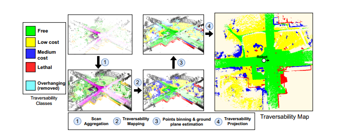
原文：对于每次扫描，我们将其与过去的t扫描和未来的t扫描进行聚合，并使用步长s构建一个更大的点集。我们将t设置为足够大的数字（例如71），以获得机器人周围大面积的密集可遍历性信息。这些参数可根据车辆速度和激光雷达点的密度进行调整。 对应步骤1

其中参数

sequence_length 为t 过去的t次扫描

stride 步长

for i in range(len(scan_files)):
    start_idx = i - (sequence_length // 2 * stride)
    history = []

    data_idxs = [start_idx + _ * stride for _ in range(sequence_length)]
    if data_idxs[0] < 0 or data_idxs[-1] >= len(scan_files):
        # Out of range
        continue

    for data_idx in data_idxs:
        scan_file = scan_files[data_idx]
        basename = os.path.splitext(scan_file)[0]
        scan_path = os.path.join(input_folder, "velodyne", scan_file)
        label_path = os.path.join(input_folder, "labels", basename + ".label")
        history.append((scan_path, label_path, poses[data_idx]))
    history = history[::-1]

    if len(history) < sequence_length:
        continue
    assert len(history) == sequence_length

将所有的信息存储到history中得到一个元数组 存储着

包括colormap cmap，点云文件的路径hist_scan_files，标签的路径hist_label_files和poe的路径hist_poses

将所有的信息传递给job_args

job_args.append({
    'cfg': cfg,
    'cmap': cmap,
    'scan_files': hist_scan_files,
    'label_files': hist_label_files,
    'poses': hist_poses,
})

gen_costmap这个函数用于生成costmap

async_results = [pool.apply_async(gen_costmap, (job, FLAGS.mem_frac)) for job in job_args]#利用多进程得到cosmap

scan 存储点云x，y，z，f

label存储标签

remissions 存储f

scan_ground_frame存储高度y

信息存储到history中

history.appendleft({
    "scan": scan.copy(),
    "scan_ground_frame": scan_ground_frame,
    "points": points,
    "labels": labels,
    "remissions": remissions,
    "pose": poses[i].copy(),
    "filename": scan_files[i]
})

keyscan表示当前的那一帧 即我们要将所有的转换给这一帧

key_scan_id = len(history) // 2
key_scan = history[key_scan_id]

首先移除掉会影响判别的移动的物体 remove_moving_objects

new_history = remove_moving_objects(history,
                                    cfg["moving_classes"],
                                    key_scan_id)

join_pointclouds 将点云聚合起来

利用左边转换 将上一帧的点云转换到这一帧的坐标下

for i, past in enumerate(history):
    diff = np.matmul(key_pose_inv, past["pose"])
    tpoints = np.matmul(diff, past["points"].T).T
    tpoints[:, 3] = past["remissions"]
    tpoints = tpoints.reshape((-1))

    npoints = past["points"].shape[0]
    end = start + npoints
    assert(npoints == past["labels"].shape[0])
    concated_points[4 * start:4 * end] = tpoints
    concated_labels[start:end] = past["labels"]
    pc_ids[start:end] = i
    start = end

得到聚合后的点云cat_points，标签cat_labels，以及是第几帧的点pc_ids

cat_points, cat_labels, pc_ids = join_pointclouds(new_history, key_scan["pose"])

然后生成cotmap create_costmap

(costmap, key_scan_postprocess_labels,
 costmap_pose) = create_costmap(cat_points, cat_labels, cfg,
                                pose=key_scan["pose"],
                                pc_ids=pc_ids,
                                key_scan_id=key_scan_id)

label利用映射转换为cost_label

mapped_labels = map_labels(labels, cfg["learning_map"])

利用这个构建map 长与宽

map_cfg = cfg["costmap"]
h = int(np.floor((map_cfg["maxy"] - map_cfg["miny"])/map_cfg["gridh"]))
w = int(np.floor((map_cfg["maxx"] - map_cfg["minx"])/map_cfg["gridw"]))

利用potprocess处理

cu_labels = postprocess(points, mapped_labels, cfg["postprocessing"])

def postprocess(points, labels, cfg):

其中利用以下代码处理点云堆叠

postprocessor = BinningPostprocess(cfg, device)

new_preds = postprocessor.process_pc(cuda_points, one_hot)
#其中one_hot[torch.arange(labels.shape[0]), cuda_labels.to(torch.long)] = 1#得到pred 结构[0,0,0,1]

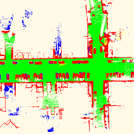
得到costmap地图

### 点云堆叠和地面高度估计

对于聚合扫描中的每个点，我们进行向下投影，以找到其在可遍历性地图上的位置x，y。因此，地图的每个x、y位置都包含一个点柱。我们通过在地图中每个x，y位置上标记为*free* and *low-cost*的点的最低z坐标上运行平均滤波核来估计地面高度地图。此高度图用作最终可通过性投影的参考。

### 可通过性投影

对于每一个点柱，我们通过将高于当地地面的点移动一定的阈值来过滤掉悬垂的障碍物，因为它们不会与机器人发生碰撞。此外，我们根据某些点离地面的高度和机器人的移动能力来调整这些点的可通过性水平。i、 e.对于大型越野车辆，标记为中等成本但非常接近当地地面的点可被视为可忽略不计，因此，将其重新映射为低成本点，与附近的其他点一样。最后，我们将每个x，y位置的最小可遍历点（即最困难点）作为最终的可遍历性标签。

理解（这一步是要利用低成本和无成本的区域来估计道路的坐标

其中BinningPostprocess 类为

  def process_pc(self, points, preds):
        ''' We assume the input prediction has 4 classes (pred.shape == nx4):
                + class 0 and 1 are traversable
                + class 2 and 3 are non-traversable
            We start off by estimating ground elavation by locally averaging z values
            of the traversable points. Then, we compute each points distance to the estimated
            ground elavation value and correct the predictions as follows:
                + (LOGIC 0) Any point outside the 2d map boundary is classified as unknown.
                + (LOGIC 1) Any point above the sky_threshold is classified as sky (a new class).
                + (LOGIC 2) Any point in class 2 that is lower than g2_threshold is labeld as class 1.
                + (LOGIC 3) Any point in class 3 that it lower than g3_threshold is labeld as class 1.
            The output is a nx5 dimensional prediction tensor.

这一段重点看一下BinningPostprocess 内部的处理

def helper():

# Usefull masks
traversable = (class_preds == 0) | (class_preds == 1)

# Project all the points
proj_ind, inrange = self.traversable_map.locs(points)
其中traversable_map
   self.traversable_map = Map2D(width, height, resx, resy) 是一个Map2D的类 
   其中 map:
                    width: 40 # map width in meters
                    height: 40 # map height in meters
                    resx: 100 # map x axis resolution
                    resy: 100 # map y axis resolution
                    将width*height的地形划分为resx*resy块
  
class Map2D(object): 
其中locs类返回位置 以num的形式 二元数组的第几个 以及返回是否在范围里
# build traversable points map and estimate ground z
            self.traversable_map.fill(points, inrange=traversable & inrange, proj_ind=proj_ind) # 返回traversable_map每个部分的z平均值
            meanz_traversable_map = self.traversable_map.apply_kernel(
                self.kernel_resw, self.kernel_resh, self.kernel_stride)
                 1 其中fill def fill(self, points, inrange=None, proj_ind=None):     
                 ''' Fill the map with the points in global coordinate system.
                 x,y will be used to to find map cell. The map cell will
                 be set by the z value.
                 Args:
                points: xyz
       			 '''
				2 其中 apply_kernel 利用滤波得到最终的图像

        # First channel holds z value, second channel is mask
        self.map = points.new_zeros((2, self.resy, self.resx)) #map 中 第一通道是z值 第二通道是mask

groundz, valid_groundz, inrange = meanz_traversable_map.query(points)
elevations = points[:, 2] - groundz

return valid_groundz, inrange, elevations, class_preds
#最终返回 mask（bool） 每个点对应的地图坐标 每个点的高度（减去地面） 预测的类别

以上是def helper(): 的处理过程

valid_groundz, inrange, elevations, class_preds = helper()
        ### Copy the original preds matrix and update it
        new_preds = preds.detach().clone()
        ## LOGIC 0: Anything outside the meanz traversable map is labeled as unknown
        new_preds[~inrange] = 0.0 # inrange 表示是否在范围内
                
                
         
        
        ## mask for the labels that might get updated
         class2 = (class_preds == 2) & valid_groundz # if it is not valid it is not inrange either
        class3 = (class_preds == 3) & valid_groundz
        nontraversable = class2 | class3
        #这里首先取出class2和class3的点
        
        
        
        

下面考虑以下四个逻辑预处理我们的点云

0是点在考虑的map外

1 是指 超过天空的阈值记为天空

2是指class2中的点低于g2_threshold阈值的转变为class1

3是指class3中的点低于g3_threshold阈值的转变为class1

最终输出一个n*5的预测值 （new_preds: tensor of corrected predictions with shape (nx5) (original classes + sky)

以上class BinningPostprocess(object): 结束

    _, new_labels = new_preds.max(axis=1)

    unknown = new_preds.sum(axis=1) == 0

    # unknown points are labeled as -1
    new_labels[unknown] = -1

torch.cuda.empty_cache()
return new_labels
#postprocess 返回处理过后的点云坐标label

这样处理的到分类

cu_labels = postprocess(points, mapped_labels, cfg["postprocessing"])

新的标签存储在cu_labels

转化为tensor数组 mapped_labels

然后投影，得到图的具体位置坐标

    valid = (cu_labels < 4) & (cu_labels >= 0)
    points = points[valid.cpu().numpy()]
    mapped_labels = cu_labels[valid].cpu().numpy()
# 取出所有的点
## projection
j_inds = np.floor((points[:, 0] - map_cfg["minx"]
                   ) / map_cfg["gridw"]).astype(np.int32)
i_inds = np.floor((points[:, 1] - map_cfg["miny"]
                   ) / map_cfg["gridh"]).astype(np.int32)

inrange = (i_inds >= 0) & (i_inds < h) & (j_inds >= 0) & (j_inds < w)

i_inds, j_inds, mapped_labels = [x[inrange] for x in [i_inds, j_inds,
                                                  mapped_labels]] # 对于每一个在地图范围内的点 inrange 每个点取出来操作

利用规则填充costmap 规则 high-cost 覆盖low-cost

# Assume that cost of class j > cost of class i if j > i
# Project the points down. Higher-cost classes overwrite low-cost classes.
costmap = np.ones((h, w), np.uint8) * 255
for l in [0, 1, 2, 3]:
    hist, _, _ = np.histogram2d(i_inds[mapped_labels == l],
                                j_inds[mapped_labels == l],
                                bins=(h, w),
                                range=((0, h), (0, w)))
    costmap[hist != 0] = l# 得到costmap 

注 https://blog.csdn.net/h201601060805/article/details/108546449

numpy的histogram2d()函数详解

这个函数可以做什么？
这个函数可以把两个二维数组，做出它的直方图出来。
什么叫做直方图：比如两个数组(A,B)都是5x5大小的，两个数组的元素都只有三个数字0,1，2
这时候得到的一个数组就是3x3的数组
(((0,0)的数量，(0,1)的数量，(0,2)的数量)，
((1,0)的数量，(1,1)的数量，(1,2)的数量)，
((2,0)的数量，(2,1)的数量，(2,2)的数量))
解释一下最里面这个(0,0)之类的
(A的位置是0，B在相同位置也是0)

得到key_can的costmap

#### extract postprocessed labels only for the key scan
if pc_ids is not None and key_scan_id >= 0:
    key_labels_ = cu_labels[pc_ids[not_void] == key_scan_id]

    scan_len = (pc_ids == key_scan_id).sum()
    key_labels = np.full(scan_len, -1)

    key_labels[not_void[pc_ids == key_scan_id]] = key_labels_.cpu().numpy()

    # 0,1,2,3,4 are reserved so use 5 for unknown?
    key_labels[key_labels < 0] = 5
            return costmap, key_labels.astype(np.uint32), costmap_pose #返回costmap  label 和 pose

以上 creat_costmap完成

costmap_1step, _, _ = create_costmap(points_1step, labels_1step, cfg,
                                     force_return_cmap=True)

costimg_1step = Image.fromarray(costmap_1step, mode='P')
costimg_1step.putpalette(cmap)
    return {
        'scan_ground_frame': key_scan['scan_ground_frame'],
        'labels': key_scan['labels'],
        'postprocessed_labels': key_scan_postprocess_labels,
        'costimg': costimg,
        'costimg_1step': costimg_1step,
        'pose': poses[key_scan_id],
        'costmap_pose': costmap_pose,
    }

以上 def gen_costmap 完成

for future in tqdm.tqdm(async_results):
    ret = future.get()
    ret['scan_ground_frame'].tofile(
        os.path.join(velodyne_folder, '{:05d}.bin'.format(counter)))
    ret["labels"].tofile(
        os.path.join(velodyne_labels_folder, '{:05d}.label'.format(counter)))
    ret['postprocessed_labels'].tofile(
        os.path.join(velodyne_pp_labels_folder, '{:05d}.label'.format(counter)))
    ret['costimg'].save(
        os.path.join(labels_folder, "{:05d}.png".format(counter)))
    ret['costimg_1step'].save(
        os.path.join(labels_1step_folder, "{:05d}.png".format(counter)))

    all_poses.append(ret['pose'][:3])
    all_costmap_poses.append(ret['costmap_pose'][:2])
    counter += 1

counters[folder] = [start_counter, counter] 
#保存数据

数据的样例

bev_1step_labels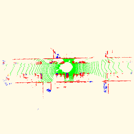

bev_labels

    all_poses.append(ret['pose'][:3])
    all_costmap_poses.append(ret['costmap_pose'][:2])
    counter += 1

counters[folder] = [start_counter, counter]

这个用于记录序号 多少到多少分别是第几序列的

semantic_bevnet-main\tools\convert_dataset.py 用于生成数据集

以上 数据生成部分完成