


week 19 GAN3
摘要
本文主要讨论了生成式对抗神经网络。首先,本文介绍了GAN训练困难性以及其在训练过程中可能出现的问题。在此基础下,本文阐述了一种可以更好评估网络的标准——Fréchet Inception Distance(FID)。此外,本文简要介绍了Conditional GAN的各种应用以及大致框架。其次本文展示了题为GANs Trained by a Two Time-Scale Update Rule Converge to a Local Nash Equilibrium的论文主要内容。这篇论文提出了双时间尺度更新规则(TTUR),并证明了使用Adam和TTUR训练GAN的收敛性。同时,该文设计了一系列实验用于评估该方法的优越性并在实验中引入了FID作为评估标准。最后,本文基于pytorch实现了Diffusion并用于绘制S型曲线。
Abstract
This article focuses on GAN. First of all, this article introduces the difficulty of GAN training and the problems that may arise during its training. On this basis, this article elaborates on a standard that can better evaluate networks—Fréchet Inception Distance(FID). In addition, this article briefly introduces the various applications of Conditional GAN and the general framework. Secondly, this paper presents the main content of the paper entitled GANs Trained by a Two Time-Scale Update Rule Converge to a Local Nash Equilibrium. This paper proposes a two time-scale update rule (TTUR) and demonstrates the convergence of training GANs using Adam and TTUR. At the same time, this paper designs a series of experiments to evaluate the superiority of the method, and introduces FID as the evaluation criterion in the experiments. Finally, this article implements Diffusion model based on pytorch and plot S-shaped curves wirh it.
一、李宏毅机器学习——GAN3
1. Introduce
max D ∈ 1 − L i p s c h i t z { E y ∼ P d a t a [ D ( y ) ] − E y ∼ P G [ D ( y ) ] } \max_{D\in1-Lipschitz}\{E_{y\sim P_{data}}[D(y)]-E_{y\sim P_G[D(y)]}\} D∈1−Lipschitzmax{Ey∼Pdata[D(y)]−Ey∼PG[D(y)]}
上述是上节中WGAN的目标公式,而在此思路下,效果最好的神经网络是SNGAN
尽管有WGAN,但GAN仍然难以训练。由于两者在训练过程中是相互对抗的,当一者收敛时(但效果不佳),另一个也将收敛。
以下是几种改进训练过程的tips

2. Difficulty in GAN training
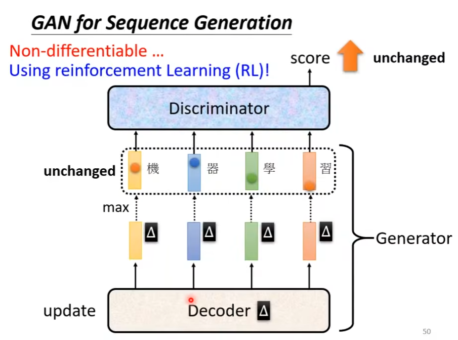
在训练GAN语言模型时,通常Discriminator会难以训练。这是因为当改变decoder时,网络内部的token可能发生较大的变化,但generator 的输出结果可能并没有变动。在这种情况下,discriminator并不会变化,此时其无需修改。
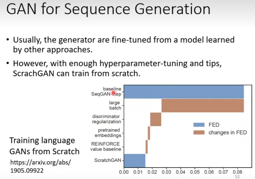
前文描述了GAN难以训练的原因,但GAN仍然可以通过多种pretrain方法来降低训练难度。Training language GANs from Scratch中给出了多种pretrain方法并将其与文中的baseline比较得出了每个方法对于GAN的提升幅度。
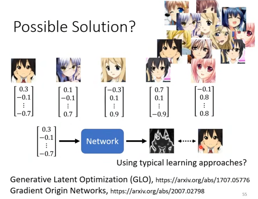
以下还提供了几个有价值的生成式模型,并提供了链接(GAN原文在week17已经讨论,故不在此处给出链接)

当然也可以按照一定规律为图片匹配one-hot vector,从而增强模型的效果,下图给出了大致过程与文章链接
3. Evaluation of Generation
在没有有效方法以前,通常使用人为评价标准。而在作业6中,使用动漫人脸探测作为评价标准,在一张图片中抓到的人脸越多,则说明该生成器的效果更加。但该探测器仅对作业6生效
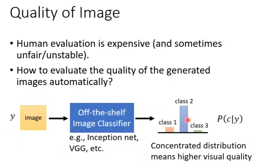
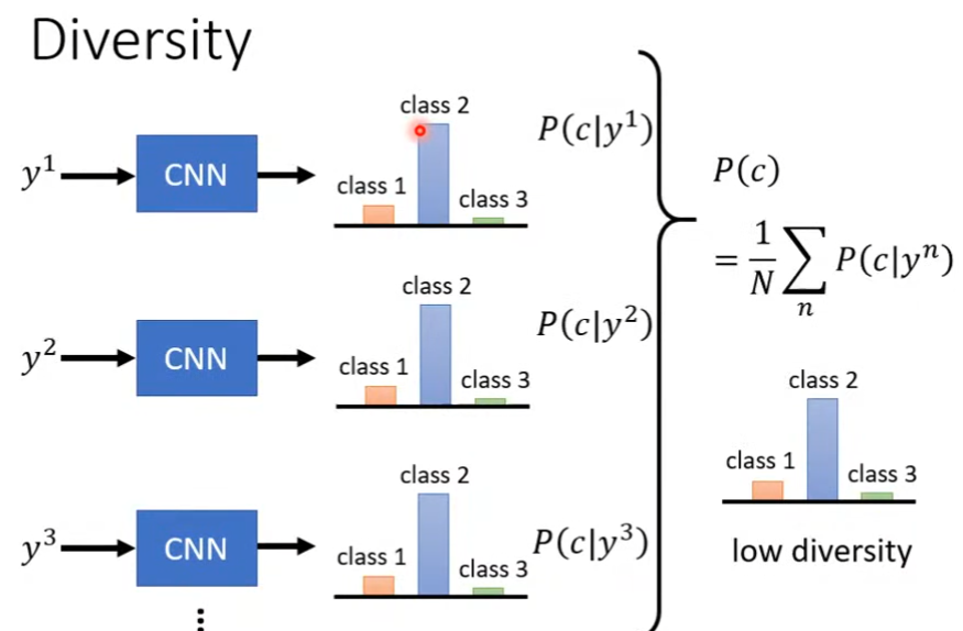
另一种方法是再训练一个影像分类模型,将图像输入模型,模型输出图像属于各个类别的概率分布。当概率分布较为集中时,意味着分类器能够较为清晰的辨别出图像,即生成器能够生成易于辨别的图像。
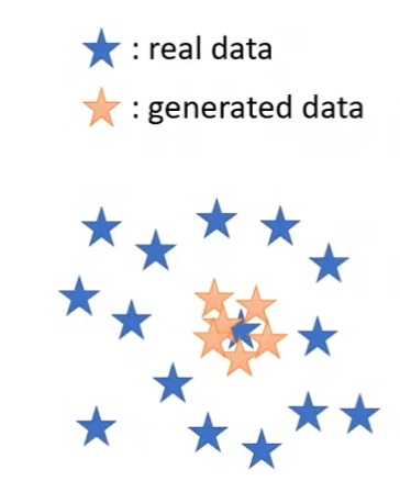
但仅使用上述方法是不可行的,可能出现mode collapse的问题。该问题是指模型生成的图像在分布上趋向于围绕单一数据点,或者仅分布在一类数据点周围。
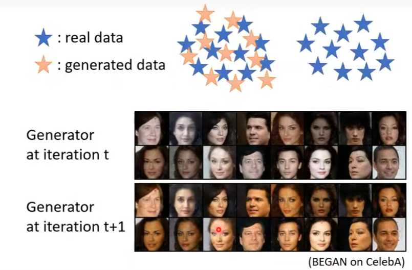
还有另一种更难以侦测的问题,mode dropping。在单一iteration内该问题并不明显,但在进行一次迭代后,可能会出现下图中的情况,这意味着模型并不稳定。其分布如下图所示
对于mode collapse,可以让生成器生成一个批次的图片,使用分类器处理这些图片,然后将分类器输出
P
(
c
∣
y
i
)
P(c|y^i)
P(c∣yi)的分布取平均
P
(
c
)
P(c)
P(c)。若结果集中在一个类别上,那么意味着该生成器的结果丰富度较低。相反,若其丰富度较高,则均值分布应该是在各个类别上较为平均分布的。
P
(
c
)
=
1
N
∑
n
P
(
c
∣
y
n
)
P(c)=\frac1N\sum_{n}P(c|y^n)
P(c)=N1n∑P(c∣yn)
基于上述思路有inception score(IS),该评估标准对质量和丰富度均有要求,当两者均较大时,IS较大。但对于人脸识别任务(HW6),由于其识别的目标均是人脸,尽管人物的各项特征可能有所不同,但是对于IS标准而言其丰富度仍是较低的,因此该任务不适合使用该评价标准。
下图描述了分布集中,丰富度较低的情况。
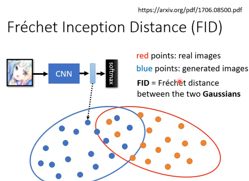
Fréchet Inception Distance(FID)
相对IS,FID使用卷积神经网络在softmax之前的vector,该向量的维数相较于softmax输出的概率分布更高。因此该向量可以更充分反应图像的特征,例如在遇到上文中的mode dropping情况时,该向量会因为迭代后人的面部肤色变化而改变,FID则通过变化推断出生成器分布可能发生了mode dropping。
而从计算角度来解释,假定下图中红色点代表cnn输出的真实图片的特征向量在特征空间内的分布情况,而蓝色则代表生成图片。FID要做的是计算两个高斯分布之间的Fréchet Distance
但该评价标准也有缺点,例如特征空间内的分布可能不是高斯分布,又或者不太确定生成图片的数量,太少不能很好的反应分布,而太多会浪费算量。上述原因会导致FID可能无法精确的评估模型,因此在HW6中需要同时考虑在探测器分辨出的人脸数量以及FID。
下图使用FID评估各种网络架构,各个架构均使用相同的网络结构,但使用不同的random seed在large-scale dataset上训练。可以看出GAN的loss分布范围较大,而VAE相对稳定,但部分GAN的下限要比VAE低。然而由于该研究使用了相同的网络架构,而各个网络适应的加过不同,可能导致结果出现偏差。
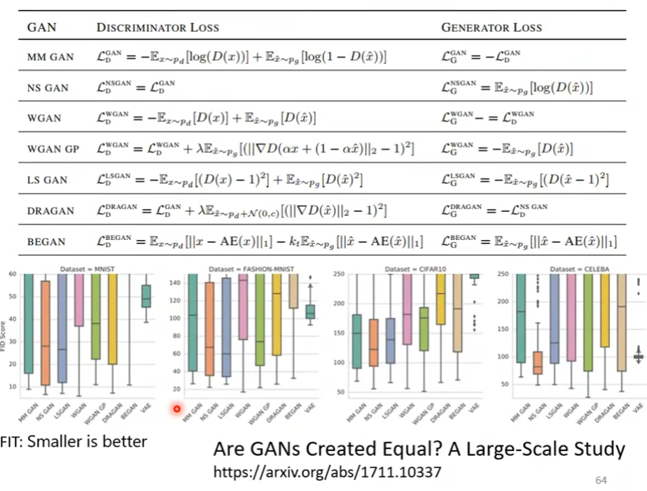
除了上文中提到的问题以外,GAN还可能生成真实数据差异不大或者其翻转。这时FID很低,但评估无效,因此GAN还需要更多评价标准。下图的论文系统性的讨论了GAN的评价标准
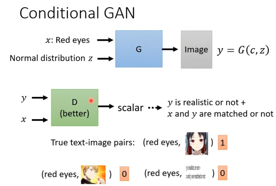
4. Conditional Generation
相较于non-conditional generation,该类网络使用输入特征x以及简单分布z作为网络输入。
相应的,辨别器也应当作出改变,因为non-conditional的分辨器仅需要考虑生成的图片是否和输入特征x相匹配。该分辨器的输入应当是生成图片y和x,输出是y是否真实以及x和y是否匹配。
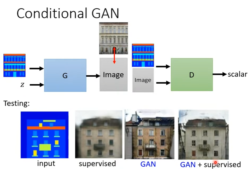
conditional GAN除了上文中的text to image以外,还可以是pix2pix。在这类任务上,使用监督学习可以使得生成图片的结构大致相似,而使用GAN可以生成更加真实的图片。因此可以将二者同时使用
此外,还有很多可以使用GAN完成的任务,例如输入声音生成图片,或是根据输入的图片以及声音让图片动起来。
二、文献阅读
1. 题目
题目:GANs Trained by a Two Time-Scale Update Rule Converge to a Local Nash Equilibrium
作者:Martin Heusel, Hubert Ramsauer, Thomas Unterthiner, Bernhard Nessler, Sepp Hochreiter
发布:NIPS2017
2. abstract
该文提出了一种两时间尺度更新规则(TTUR),用于在任意GAN损失函数上使用随机梯度下降来训练GAN。该文证明了TTUR在温和假设下收敛于稳态局部Nash均匀。此外,该文引入了Fréchet Inception Distance(FID)作为评估标准,它比 Inception Score 更好地捕获了生成图像与真实图像的相似性。
This article proposes a two time-scale update rule (TTUR) for training GANs with stochastic gradient descent on arbitrary GAN loss functions. It also prove that the TTUR converges under mild assumptions to a stationary local Nash equilibrium. In addition, this article introduces the ‘Fréchet Inception Distance”(FID) as an evaluation criterion, which captures the similarity of generated images to real ones better than the Inception Score.
3. 文章主要内容
3.1 基于GANs的双时间尺度更新规则
假定有判别器
D
(
.
;
w
)
D(.;w)
D(.;w)以及生成器
G
(
.
;
θ
)
G(.;\theta)
G(.;θ),其中
w
,
θ
w,\theta
w,θ均是参数向量;训练基于随机梯度,判别器损失函数
L
D
\mathcal L_D
LD的随机梯度为
g
~
(
θ
;
w
)
\tilde g(\theta;w)
g~(θ;w),生成器损失函数
L
G
\mathcal L_G
LG的随机梯度为
h
~
(
θ
,
w
)
\tilde h(\theta,w)
h~(θ,w)。两个损失函数不一定相关。若真实梯度是
g
(
θ
,
w
)
=
∇
w
L
D
,
h
(
θ
,
w
)
=
∇
θ
L
G
g(\theta,w)=\nabla_w\mathcal L_D,h(\theta,w)=\nabla_\theta\mathcal L_G
g(θ,w)=∇wLD,h(θ,w)=∇θLG,则定义梯度
g
~
(
θ
,
w
)
=
g
(
θ
,
w
)
+
M
(
w
)
\tilde g(\theta,w)=g(\theta,w)+M(w)
g~(θ,w)=g(θ,w)+M(w)和
h
~
(
θ
,
w
)
=
h
(
θ
,
w
)
+
M
(
θ
)
\tilde h(\theta,w)=h(\theta,w)+M(\theta)
h~(θ,w)=h(θ,w)+M(θ),随机变量为M(w)和
M
(
θ
)
M(\theta)
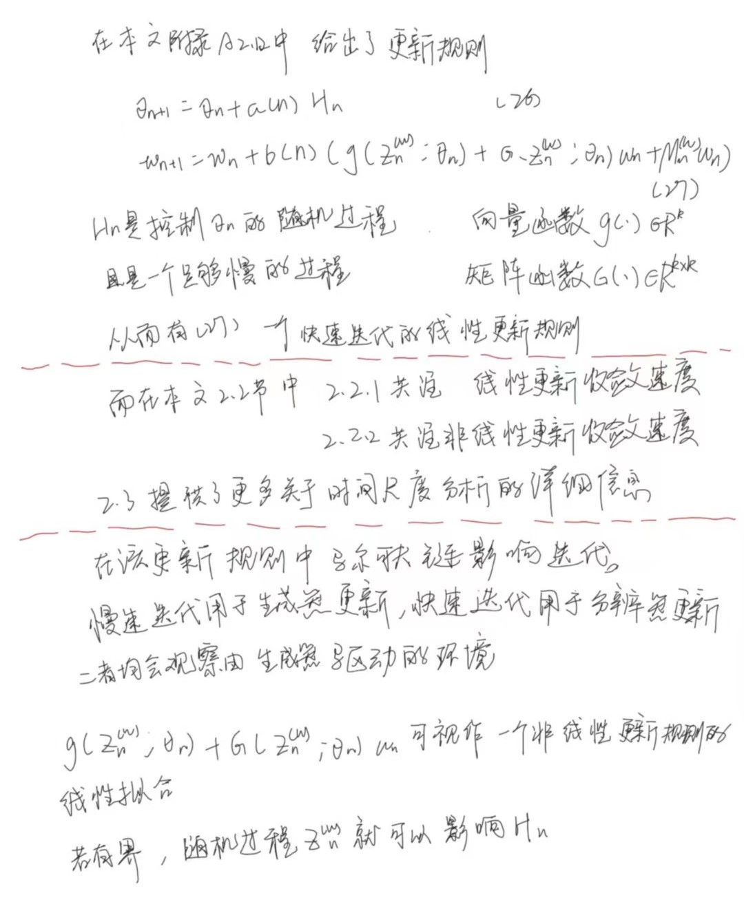
M(θ)。通过双尺度随机近似算法来分析GAN的收敛性。对于TTUR,分别使用学习率b(n)和a(n)进行判别器和生成器的更新:
w
n
+
1
=
w
n
+
b
(
n
)
(
g
(
θ
n
,
w
n
)
+
M
n
(
w
)
)
)
,
θ
n
+
1
=
θ
n
+
a
(
n
)
(
h
(
θ
n
,
w
n
)
+
M
n
(
θ
)
)
(1)
w_{n+1}=w_n+b(n)(g(\theta_n,w_n)+M_n^{(w)})),\theta_{n+1}=\theta_n+a(n)(h(\theta_n,w_n)+M_n^{(\theta)}) \tag{1}
wn+1=wn+b(n)(g(θn,wn)+Mn(w))),θn+1=θn+a(n)(h(θn,wn)+Mn(θ))(1)
上述过程证明了TTUR可收敛,而下图给出了其具体的线性更新规则以及各部分的含义(不包括上文已经给出的部分)。
3.2 Adam确保TTUR收敛
3.2.1 使用Adam以降低收敛至局域最小的概率
作者计划使用Adam随机拟合以规避mode collapsing(课程部分已经给出,不再赘述)。
在作者的描述中,Adam被看作具有摩擦力的的重球(HBF),因其对过去梯度进行平均。该均值能在生成器能够抵抗被推入小区域时提供速度。
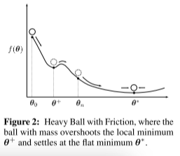
简单来说,如上图,Adam能够在 θ + \theta^+ θ+位置为生成器提供速度,使得其能够脱离局部最极小值,并进一步达到平滑最小值 θ ∗ \theta^* θ∗
3.2.2 分析是否收敛的过程
第n步的Adam更新规则,
- 学习率为a
- 梯度 ∇ f ( θ n − 1 ) \nabla f(\theta_{n-1}) ∇f(θn−1)
- β 1 \beta_1 β1,第一次估计的指数衰减率
- β 2 \beta_2 β2,第二次估计的指数衰减率
- ϵ \epsilon ϵ,防止在计算过程中除以零
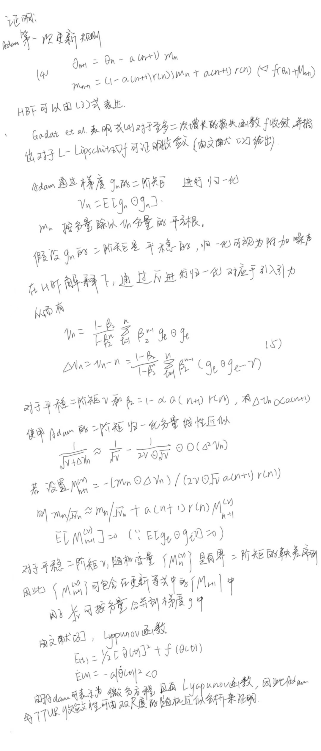
g n ← ∇ f ( θ n − 1 ) m n ← ( β 1 / ( 1 − β 1 n ) ) m n − 1 + ( ( 1 − β 1 ) / ( 1 − β 1 n ) ) g n v n ← ( β 2 / ( 1 − β 2 n ) ) v n − 1 + ( ( 1 − β 2 ) / ( 1 − β 2 n ) ) g n ⊙ g n θ n ← θ n − 1 − a m n / ( v n + ϵ ) (2) g_n\leftarrow \nabla f(\theta_{n-1})\\ m_n\leftarrow (\beta_1/(1-\beta_1^n))m_{n-1}+((1-\beta_1)/(1-\beta_1^n))g_n\\ v_n\leftarrow(\beta_2/(1-\beta_2^n))v_{n-1}+((1-\beta_2)/(1-\beta_2^n))g_n\odot g_n\\ \theta_n\leftarrow \theta_{n-1}-am_n/(\sqrt v_n+\epsilon) \tag{2} gn←∇f(θn−1)mn←(β1/(1−β1n))mn−1+((1−β1)/(1−β1n))gnvn←(β2/(1−β2n))vn−1+((1−β2)/(1−β2n))gn⊙gnθn←θn−1−amn/(vn+ϵ)(2)
为了使用ODE思想描述Adam,从而使用证明使用TTUR和Adam作为GAN的构建能够使得该网络收敛。首先引入阻尼系数 a ( n ) = a n − τ f o r τ ∈ ( 0 , 1 ] a(n)=a_n^{-\tau}\ for\ \tau\in(0,1] a(n)=an−τ for τ∈(0,1]。其次,令指数记忆 r ( n ) = r r(n)=r r(n)=r,多项式记忆 r ( n ) = r / ∑ l = 1 n a ( l ) r(n)=r/\sum_{l=1}^na(l) r(n)=r/∑l=1na(l)
Theorem2:若使用Adam作为优化器,且
β
1
=
1
−
a
(
n
+
1
)
r
(
n
)
,
β
2
=
1
−
α
a
(
n
+
1
)
r
(
n
)
\beta_1=1-a(n+1)r(n),\beta_2=1-\alpha a(n+1)r(n)
β1=1−a(n+1)r(n),β2=1−αa(n+1)r(n),同时
∇
f
\nabla f
∇f是下界连续可微目标f的完整梯度,则对于梯度的平稳二阶矩,Adam遵循带有HBF的微分方程
θ
t
¨
+
a
(
t
)
θ
t
˙
+
∇
f
(
θ
t
)
=
0
(3)
\ddot {\theta_t}+a(t)\dot {\theta_t}+\nabla f(\theta_t)=\bf 0 \tag{3}
θt¨+a(t)θt˙+∇f(θt)=0(3)
Adam收敛于L-Lipschitz梯度
∇
f
\nabla f
∇f
证明过程如下
4. 文献解读
4.1 Introduction
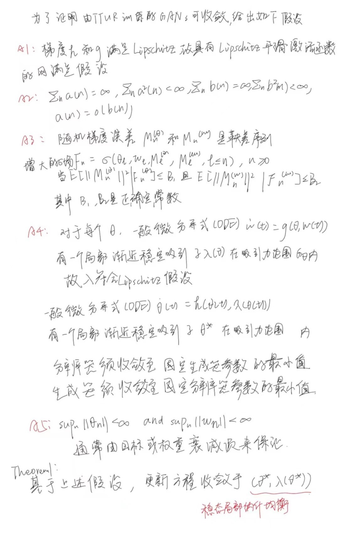
由于训练GAN是一种博弈,其解决方案是nash均衡,因此梯度下降可能无法使其收敛。因为梯度下降是一种局部优化方法,相应的其只能找到局部纳什均衡。作者将参数空间中某个点周围存在一个局部邻域,其中生成器和判别器都不能单方面减少各自的损失,称之为局部纳什均衡。即当对抗双方中的一个停止提升时,另一方也无法提升。
作者证明了使用TTUR训练的GAN在训练时会收敛至稳态纳什均衡。作者还将Adam描述为一个具有摩擦力的重球,从而使用二阶微分方程来进行描述。最后使用TTUR和Adam训练GAN,并评估了FID作为评价标准的效果,结果证明其效果由于IS(Inception Score)。
tips:纳什均衡的定义:在博弈G=﹛S1,…,Sn:u1,…,un﹜中,如果由各个博弈方的各一个策略组成的某个策略组合(s1 *,…,sn *)中,任一博弈方i的策略si *,都是对其余博弈方策略的组合(s1 *,…s *i-1,s *i+1,…,sn *)的最佳对策,也即ui(s1 *,…s *i-1,si *,s *i+1,…,sn *)≥ui(s1 *,…s *i-1,sij *,s *i+1,…,sn *)对任意sij∈Si都成立,则称(s1 *,…,sn *)为G的一个纳什均衡。
4.2 创新点
- 给出了新的双时间尺度的更新规则
- 证明了TTUR能够使得GAN收敛于稳态纳什均衡
- 使用TTUR和Adam训练GAN至稳态纳什均衡
- 使用FID和IS评估,并证明了FID在该任务上的优越性
4.3 实验过程
4.3.1 性能指标
FID公式如下[4]
d
2
(
(
m
,
C
)
,
(
m
w
,
C
w
)
)
=
∣
∣
m
−
m
w
∣
∣
2
2
+
Tr
(
C
+
C
w
−
2
(
C
C
w
)
1
2
)
(6)
d^2((m,C),(m_w,C_w))=||m-m_w||_2^2+\text{Tr}(C+C_w-2(CC_w)^{\frac12}) \tag{6}
d2((m,C),(mw,Cw))=∣∣m−mw∣∣22+Tr(C+Cw−2(CCw)21)(6)
下图评估了FID,左上Gaussian noise,上中Gaussian blur,右上implanted black rectangles
左下swirled images,下中salt and pepper noise(黑白噪点),右下CelebA dataset, ImageNet images混合
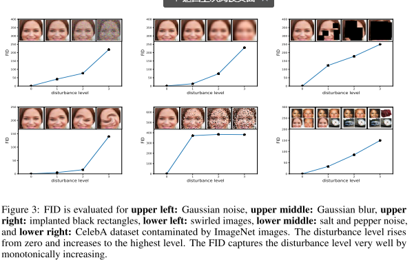
根据上图FID可以很好的捕捉干扰水平,在实验中可以使用FID来评估GAN的性能
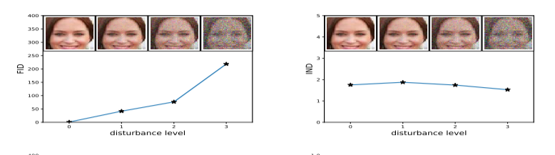
下图对比了使用FID和使用IS评估的效果,图片添加高斯噪声。显然IS没有明显变化,但FID随着噪声强度增大明显增大。该文还提供了其他各种噪声类型的对比情况,不再赘述。
4.3.2 模型选择与评估
将 GAN 的两种时间尺度更新规则(TTUR)与原始 GAN 训练进行比较,看看 TTUR 是否提高了 GAN 的收敛速度和性能。该文选择 Adam 随机优化来降低模式崩溃的风险。 对于每个实验,通过 FID 或 Jensen-Shannon 散度 (JSD) 的减小来表明学习率在合理区间。当最佳模型的 FID 或 JSD不再减小时,将停止训练的时间点固定为更新步骤。
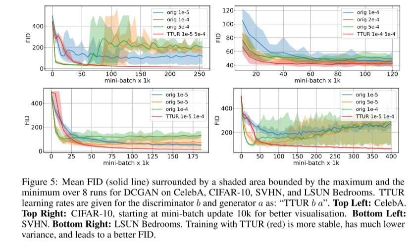
对于某些模型,FID 在某个时间点出现发散或开始增加。如下图。
- 实线周围的区域标识DCGAN在各个数据集上的8次运行内的最大值最小值区间。
- 实线为FID均值
- “orig 1e-5”,表示原始GAN,学习率为1e-5。
- "TTUR 1e-5 5e-4"表示TTUR模型,分辨器学习率1e-5,生成器学习率1e-4。
- 四张图分别表示在CelebA、CIFAR-10、SVHN、LSUN Bedrooms各个数据集上的运行效果。
由TTUR训练的模型更加稳定,且方差更小,有一个较好的FID。
4.3.3 图像数据上的WGAN-GP
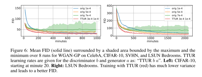
使用 WGAN-GP 图像模型通过 CIFAR-10 和 LSUN Bedrooms 数据集测试 TTUR。每次生成器更新时TTUR更新分辨器一次,故将训练进度与时间刻度保持一致。TTUR可为判别器使用更大学习率,因为其可以稳定学习。下图显示了使用原始学习方法和TTUR方法进行学习期间的FID
规则与上图大致相同,故不再赘述,左侧为CIFAR-10,右侧为LSUN Bedrooms。TTUR也表现出了更稳定更好的效果。
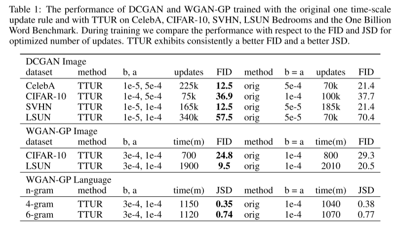
下表显示了采用TTUR和单一时间尺度训练的最佳FID,并标识了优化迭代次数和学习率,以进行比较。TTUR的FID相较单一尺度更低。
tip:下表分为三部分,从上到下,第一部分在图像数据上使用DCGAN(4.3.2),第二部分在图像数据上使用WGAN-GP(4.3.3),第三部分在语言数据上使用WGAN-GP(4.3.4)
4.3.4 语言数据上的WGAN-GP
使用十亿字基准(One Billion Word Benchmark)用于评估 WGAN-GP 上的 TTUR。由于 FID 准则仅适用于图像,因此使用JSD来测量性能。每次生成器更新,TTUR 仅更新分辨器一次,因此我们将训练进度与时间刻度保持一致。
上表中第三部分为最佳时间步长的最佳 JSD,其中 TTUR 优于标准训练两项措施。 TTUR 在 6-gram 统计数据上相对于原始训练的改进表明,TTUR 能够学习生成更微妙的伪词,更类似于真实单词。
下图显示了 4 和 6 粒度的单词评估的原始训练和 TTUR 训练十次运行的归一化平均 JSD。(左侧4-gram,右侧6-gram)

4.4 结论
该文引入了双时间尺度更新规则(TTUR),且证明了该规则可收敛至稳态局部纳什均衡。然后证明了用TTUR和Adam训练的GAN收敛至稳态局部纳什均衡。引入了FID,并使用实验以及理论上证明了其比IS更能捕捉生成图像和真实图像的相似性。最后使用DCGAN、WGAN-GP网络在多个不同类别的数据集上使用FID或者JSD证明了文中方法的优越性。
三、pytorch实现diffusion模型
关于该模型的原理将由另一篇文章介绍,以下为实验记录
1. 实验结果
第一个批次时的图像
最后一个批次的图像
2. 实验代码
import matplotlib.pyplot as plt
import numpy as np
from sklearn.datasets import make_s_curve
import torch
import torch
import torch.nn as nn
import io
from PIL import Image
# 生成一万个点,得到s curve
s_curve,_ = make_s_curve(10**4,noise=0.1)
s_curve = s_curve[:,[0,2]]/10.0
print("shape of s:",np.shape(s_curve))
data = s_curve.T
fig,ax = plt.subplots()
ax.scatter(*data,color='blue',edgecolor='white');
ax.axis('off')
#当成一个数据集
dataset = torch.Tensor(s_curve).float()
#画出 s curve
plt.show()
#确定超参数的值
num_steps = 100 #可由beta值估算
#制定每一步的beta,beta按照时间从小到大变化
betas = torch.linspace(-6,6,num_steps)
betas = torch.sigmoid(betas)*(0.5e-2 - 1e-5)+1e-5
#计算alpha、alpha_prod、alpha_prod_previous、alpha_bar_sqrt等变量的值
alphas = 1-betas
# alpha连乘
alphas_prod = torch.cumprod(alphas,0)
#从第一项开始,第0项另乘1???
alphas_prod_p = torch.cat([torch.tensor([1]).float(),alphas_prod[:-1]],0)
# alphas_prod开根号
alphas_bar_sqrt = torch.sqrt(alphas_prod)
#之后公式中要用的
one_minus_alphas_bar_log = torch.log(1 - alphas_prod)
one_minus_alphas_bar_sqrt = torch.sqrt(1 - alphas_prod)
# 大小都一样,常数不需要训练
assert alphas.shape==alphas_prod.shape==alphas_prod_p.shape==\
alphas_bar_sqrt.shape==one_minus_alphas_bar_log.shape\
==one_minus_alphas_bar_sqrt.shape
print("all the same shape",betas.shape)
#给定初始,算出任意时刻采样值——正向扩散
# 计算任意时刻的x采样值,基于x_0和重参数化
def q_x(x_0, t):
"""可以基于x[0]得到任意时刻t的x[t]"""
#生成正态分布采样
noise = torch.randn_like(x_0)
#得到均值方差
alphas_t = alphas_bar_sqrt[t]
alphas_1_m_t = one_minus_alphas_bar_sqrt[t]
#根据x0求xt
return (alphas_t * x_0 + alphas_1_m_t * noise) # 在x[0]的基础上添加噪声
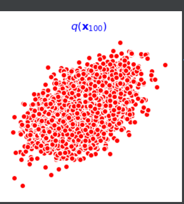
# 演示加噪过程,加噪100步情况
num_shows = 20
fig,axs = plt.subplots(2,10,figsize=(28,3))
plt.rc('text',color='black')
#共有10000个点,每个点包含两个坐标
#生成100步以内每隔5步加噪声后的图像,扩散过程散点图演示——基于x0生成条件分布采样得到xt
for i in range(num_shows):
j = i//10
k = i%10
q_i = q_x(dataset,torch.tensor([i*num_steps//num_shows])) # 生成t时刻的采样数据
axs[j,k].scatter(q_i[:,0],q_i[:,1],color='red',edgecolor='white')
axs[j,k].set_axis_off()
axs[j,k].set_title('$q(\mathbf{x}_{'+str(i*num_steps//num_shows)+'})$')
plt.show()
# 拟合逆扩散过程高斯分布模型——拟合逆扩散时的噪声
#自定义神经网络
class MLPDiffusion(nn.Module):
def __init__(self, n_steps, num_units=128):
super(MLPDiffusion, self).__init__()
self.linears = nn.ModuleList(
[
nn.Linear(2, num_units),
nn.ReLU(),
nn.Linear(num_units, num_units),
nn.ReLU(),
nn.Linear(num_units, num_units),
nn.ReLU(),
nn.Linear(num_units, 2),
]
)
self.step_embeddings = nn.ModuleList(
[
nn.Embedding(n_steps, num_units),
nn.Embedding(n_steps, num_units),
nn.Embedding(n_steps, num_units),
]
)
def forward(self, x, t):
# x = x_0
for idx, embedding_layer in enumerate(self.step_embeddings):
t_embedding = embedding_layer(t)
x = self.linears[2 * idx](x)
x += t_embedding
x = self.linears[2 * idx + 1](x)
x = self.linears[-1](x)
return x
#编写训练误差函数
def diffusion_loss_fn(model, x_0, alphas_bar_sqrt, one_minus_alphas_bar_sqrt, n_steps):
"""对任意时刻t进行采样计算loss"""
batch_size = x_0.shape[0]
# 对一个batchsize样本生成随机的时刻t,t变得随机分散一些,一个batch size里面覆盖更多的t
t = torch.randint(0, n_steps, size=(batch_size // 2,))
t = torch.cat([t, n_steps - 1 - t], dim=0)# t的形状(bz)
t = t.unsqueeze(-1)# t的形状(bz,1)
# x0的系数,根号下(alpha_bar_t)
a = alphas_bar_sqrt[t]
# eps的系数,根号下(1-alpha_bar_t)
aml = one_minus_alphas_bar_sqrt[t]
# 生成随机噪音eps
e = torch.randn_like(x_0)
# 构造模型的输入
x = x_0 * a + e * aml
# 送入模型,得到t时刻的随机噪声预测值
output = model(x, t.squeeze(-1))
# 与真实噪声一起计算误差,求平均值
return (e - output).square().mean()
#编写逆扩散采样函数
#从xt恢复x0
def p_sample_loop(model, shape, n_steps, betas, one_minus_alphas_bar_sqrt):
"""从x[T]恢复x[T-1]、x[T-2]|...x[0]"""
cur_x = torch.randn(shape)
x_seq = [cur_x]
for i in reversed(range(n_steps)):
cur_x = p_sample(model, cur_x, i, betas, one_minus_alphas_bar_sqrt)
x_seq.append(cur_x)
return x_seq
def p_sample(model, x, t, betas, one_minus_alphas_bar_sqrt):
"""从x[T]采样t时刻的重构值"""
t = torch.tensor([t])
coeff = betas[t] / one_minus_alphas_bar_sqrt[t]
eps_theta = model(x, t)
#得到均值
mean = (1 / (1 - betas[t]).sqrt()) * (x - (coeff * eps_theta))
z = torch.randn_like(x)
sigma_t = betas[t].sqrt()
#得到sample的分布
sample = mean + sigma_t * z
return (sample)
#开始训练模型,打印loss以及中间的重构效果
seed = 1234
class EMA():
"""构建一个参数平滑器"""
def __init__(self, mu=0.01):
self.mu = mu
self.shadow = {}
def register(self, name, val):
self.shadow[name] = val.clone()
def __call__(self, name, x):
assert name in self.shadow
new_average = self.mu * x + (1.0 - self.mu) * self.shadow[name]
self.shadow[name] = new_average.clone()
return new_average
print('Training model...')
batch_size = 128
# dataset放到dataloader中
dataloader = torch.utils.data.DataLoader(dataset, batch_size=batch_size, shuffle=True)
# 迭代周期
num_epoch = 4000
plt.rc('text', color='blue')
#实例化模型,传入一个数
model = MLPDiffusion(num_steps) # 输出维度是2,输入是x和step
optimizer = torch.optim.Adam(model.parameters(), lr=1e-3)
# epoch遍历
for t in range(num_epoch):
if t % 10 == 0:
print("epoch:", t)
# dataloader遍历
for idx, batch_x in enumerate(dataloader):
# 得到loss
loss = diffusion_loss_fn(model, batch_x, alphas_bar_sqrt, one_minus_alphas_bar_sqrt, num_steps)
optimizer.zero_grad()
loss.backward()
#梯度clip,保持稳定性
torch.nn.utils.clip_grad_norm_(model.parameters(), 1.)
optimizer.step()
#每100步打印效果
if (t % 100 == 0):
print(loss)
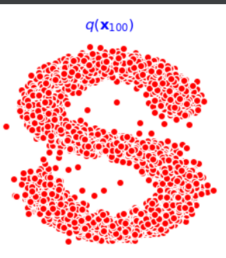
#根据参数采样一百个步骤的x,每隔十步画出来,迭代了4000个周期,逐渐更接近于原始
x_seq = p_sample_loop(model, dataset.shape, num_steps, betas, one_minus_alphas_bar_sqrt)
fig, axs = plt.subplots(1, 10, figsize=(28, 3))
for i in range(1, 11):
cur_x = x_seq[i * 10].detach()
axs[i - 1].scatter(cur_x[:, 0], cur_x[:, 1], color='red', edgecolor='white');
axs[i - 1].set_axis_off();
axs[i - 1].set_title('$q(\mathbf{x}_{' + str(i * 10) + '})$')
plt.show()
# 前向后向过程gif
imgs = []
for i in range(100):
plt.clf()
q_i = q_x(dataset, torch.tensor([i]))
plt.scatter(q_i[:, 0], q_i[:, 1], color='red', edgecolor='white', s=5);
plt.axis('off');
img_buf = io.BytesIO()
plt.savefig(img_buf, format='png')
img = Image.open(img_buf)
imgs.append(img)
plt.show()
reverse = []
for i in range(100):
plt.clf()
cur_x = x_seq[i].detach()
plt.scatter(cur_x[:, 0], cur_x[:, 1], color='red', edgecolor='white', s=5);
plt.axis('off')
img_buf = io.BytesIO()
plt.savefig(img_buf, format='png')
img = Image.open(img_buf)
reverse.append(img)
plt.show()
imgs = imgs +reverse
imgs[0].save("diffusion.gif",format='GIF',append_images=imgs,save_all=True,duration=100,loop=0)
小结
上周学习了WGAN,该模型可以降低GAN模型的训练难度,但总的来说,该模型依旧难以训练。传统的随机梯度下降算法在GAN中仅能通过Discriminator来控制整个网络。然而由于该模型的特殊性,在Discriminator输出不变的情况下,Generator网络中的参数可能有较大的变动。在文中提到的论文中验证了可以使用多种pretrain方法来降低GAN的训练难度。而在HW6中采用了另一种评估标准来降低训练难度,因为该评估标准当模型发生mode collapse、mode dropping等问题时能够提供反应。最后,本文简要介绍了conditional GAN,这也是下周计划的学习内容。
参考文献
[1] M. Heusel, H. Ramsauer, T. Unterthiner, B. Nessler, & S. Hochreiter, “gans trained by a two time-scale update rule converge to a local nash equilibrium”, 2017. https://doi.org/10.48550/arxiv.1706.08500
[2] S. Gadat, F. Panloup, and S. Saadane. Stochastic heavy ball. arXiv e-prints, arXiv:1609.04228,
2016.
[3] H. Attouch, X. Goudou, and P. Redont. The heavy ball with friction method, I. the continu-
ous dynamical system: Global exploration of the local minima of a real-valued function by
asymptotic analysis of a dissipative dynamical system. Communications in Contemporary
Mathematics, 2(1):1–34, 2000.
[4] D. C. Dowson and B. V. Landau. The Fréchet distance between multivariate normal distributions. Journal ofMultivariate Analysis, 12:450–455, 1982.


 1710
1710

 被折叠的 条评论
为什么被折叠?
被折叠的 条评论
为什么被折叠?
 到【灌水乐园】发言


