 图卷积网络GCN:结构信息的利用


原文链接:https://ai.plainenglish.io/graph-convolutional-networks-gcn-baf337d5cb6b
In this post, we’re gonna take a close look at one of the well-known Graph neural networks named GCN. First, we’ll get the intuition to see how it works, then we’ll go deeper into the maths behind it.
Why Graphs?
![Examples of graphs. (Picture from [1])](https://i-blog.csdnimg.cn/blog_migrate/93ad6ae9157347c20d9aefb8652bef18.png)
Tasks on Graphs
- Node classification: Predict a type of a given node
- Link prediction: Predict whether two nodes are linked
- Community detection: Identify densely linked clusters of nodes
- Network similarity: How similar are two (sub)networks
Machine Learning Lifecycle
In the graph, we have node features (the data of nodes) and the structure of the graph (how nodes are connected).
For the former, we can easily get the data from each node. But when it comes to the structure, it is not trivial to extract useful information from it. For example, if 2 nodes are close to one another, should we treat them differently to other pairs? How about high and low degree nodes? In fact, each specific task can consume a lot of time and effort just for Feature Engineering, i.e., to distill the structure into our features.
![Feature engineering on graphs. (Picture from [1])](https://i-blog.csdnimg.cn/blog_migrate/391bf3e2d35619fa123cc01ea9928b52.png)
It would be much better to somehow get both the node features and the structure as the input, and let the machine to figure out what information is useful by itself.
That’s why we need Graph Representation Learning.
![We want the graph can learn the “feature engineering” by itself. (Picture from [1])](https://i-blog.csdnimg.cn/blog_migrate/4ed17f8a437aa658f52a5d91a02ef7e2.png)
Graph Convolutional Networks (GCNs)
Paper: Semi-supervised Classification with Graph Convolutional Networks (2017) [3]
GCN is a type of convolutional neural network that can work directly on graphs and take advantage of their structural information.
it solves the problem of classifying nodes (such as documents) in a graph (such as a citation network), where labels are only available for a small subset of nodes (semi-supervised learning).
Main Ideas
As the name “Convolutional” suggests, the idea was from Images and then brought to Graphs. However, when Images have a fixed structure, Graphs are much more complex.
![Convolution idea from images to graphs. (Picture from [1])](https://i-blog.csdnimg.cn/blog_migrate/6673a8a66f578250b97e855bfd54d58d.png)
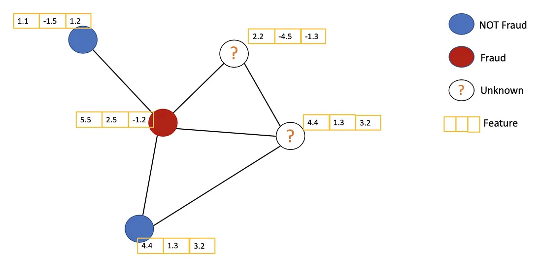
The general idea of GCN: For each node, we get the feature information from all its neighbors and of course, the feature of itself. Assume we use the average() function. We will do the same for all the nodes. Finally, we feed these average values into a neural network.
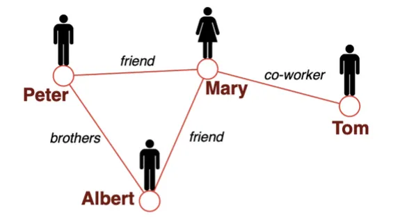
In the following figure, we have a simple example with a citation network. Each node represents a research paper, while edges are the citations. We have a pre-process step here. Instead of using the raw papers as features, we convert the papers into vectors (by using NLP embedding, e.g., tf–idf, Doc2Vec).
Let’s consider the orange node. First off, we get all the feature values of its neighbors, including itself, then take the average. The result will be passed through a neural network to return a resulting vector.
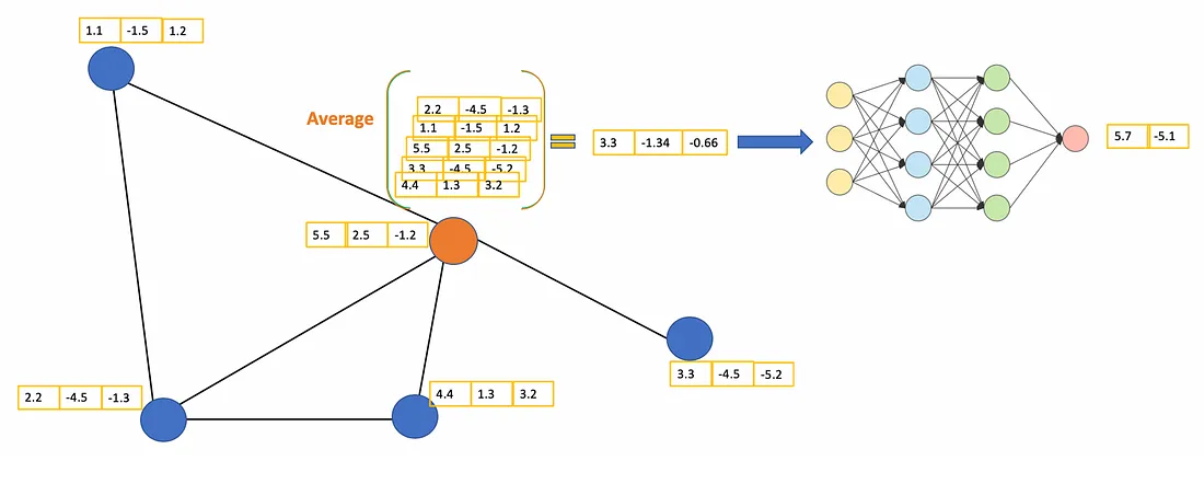
In practice, we can use more sophisticated aggregate functions rather than the average function. We can also stack more layers on top of each other to get a deeper GCN. The output of a layer will be treated as the input for the next layer.
Let’s take a closer look at the maths to see how it really works.
Intuition and the Maths behind
First, we need some notations:
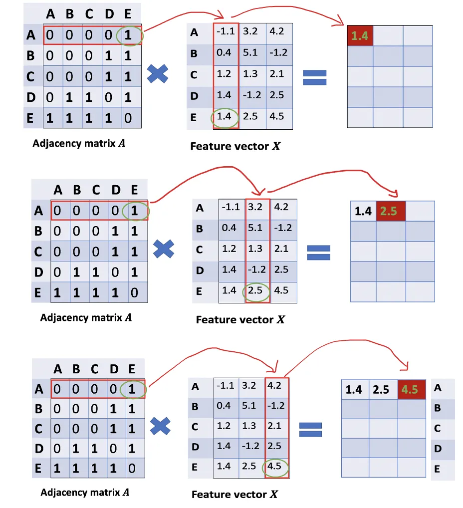
Given an undirected graph G = ( V , E ) G = (V, E) G=(V,E) with N N N nodes v i ∈ V v_i \in V vi∈V, edges ( v i , v j ) ∈ E (v_i, v_j) \in E (vi,vj)∈E, an adjacency matrix A ∈ R N × N A \in R^{N×N} A∈RN×N (binary or weighted), degree matrix D i i = ∑ j A i j D_{ii} = \sum_j Α_{ij} Dii=∑jAij and feature vector matrix X ∈ R N × C X \in R^{N×C} X∈RN×C (N is #nodes, C is the #dimensions of a feature vector).
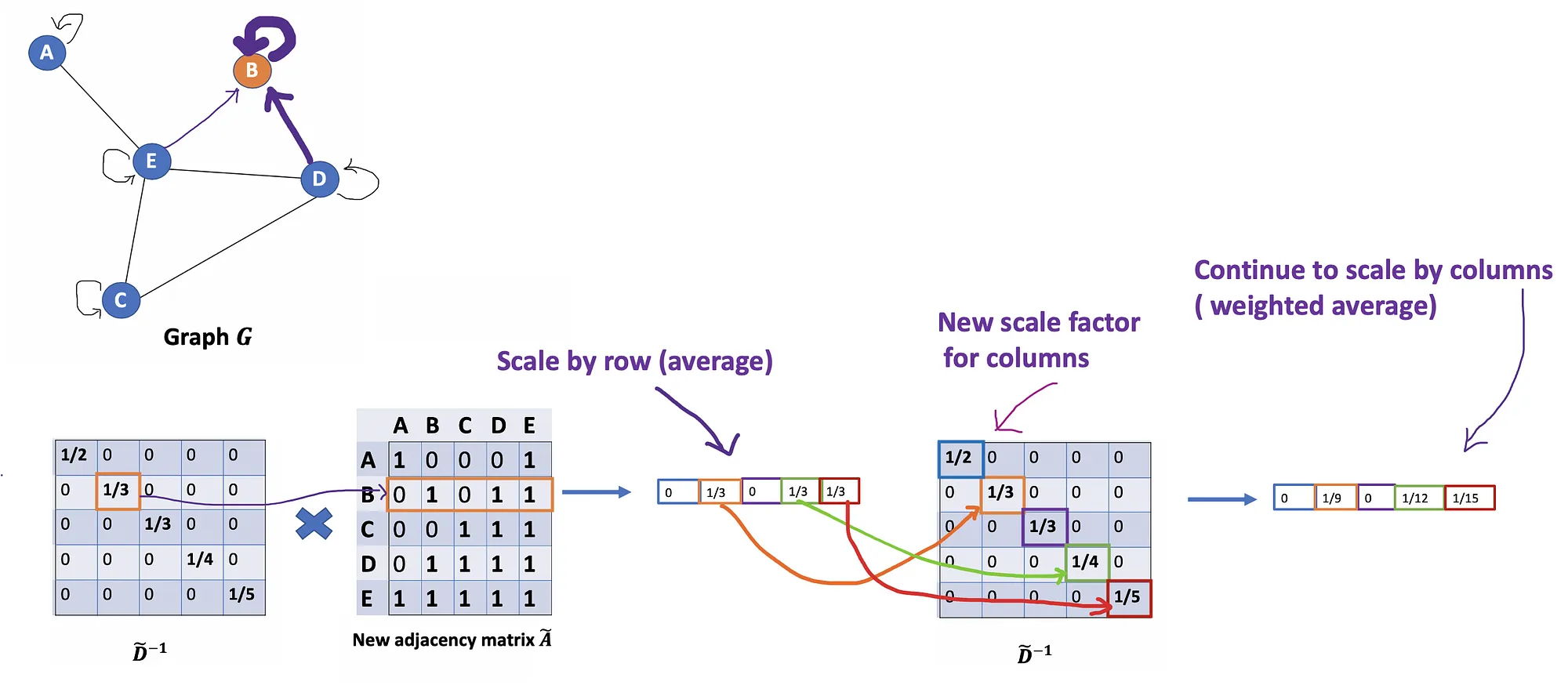
Let’s consider a graph G as below.
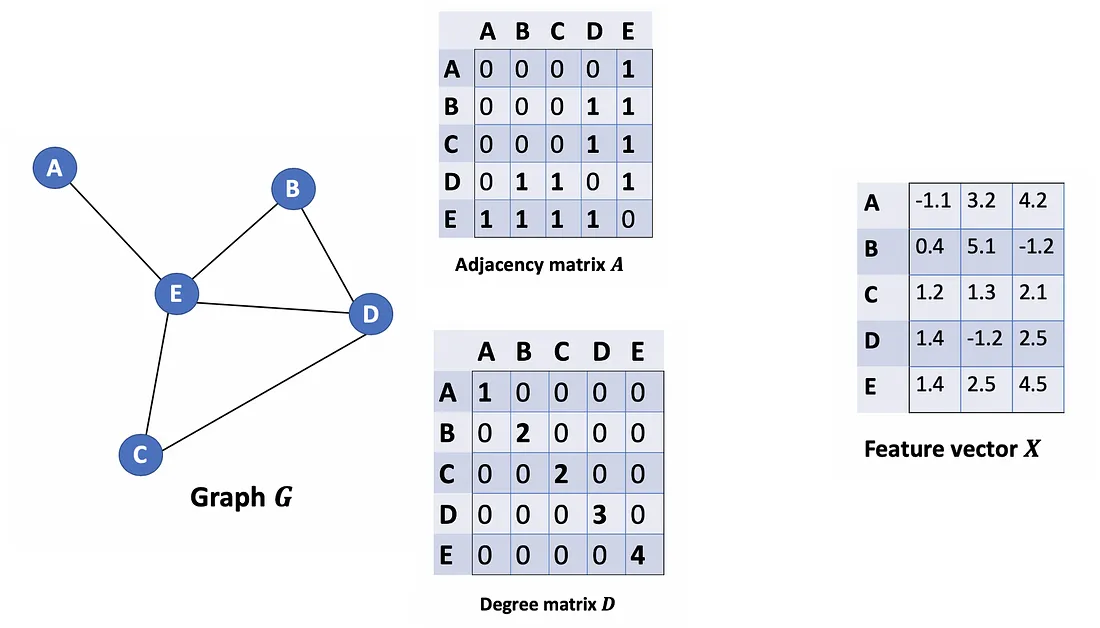
How can we get all the feature values from neighbors for each node? The solution lies in the multiplication of A and X.
Take a look at the first row of the adjacency matrix, we see that node A has a connection to E. The first row of the resulting matrix is the feature vector of E, which A connects to (Figure below). Similarly, the second row of the resulting matrix is the sum of feature vectors of D and E. By doing this, we can get the sum of all neighbors’ vectors.
There are still some things that need to improve here.
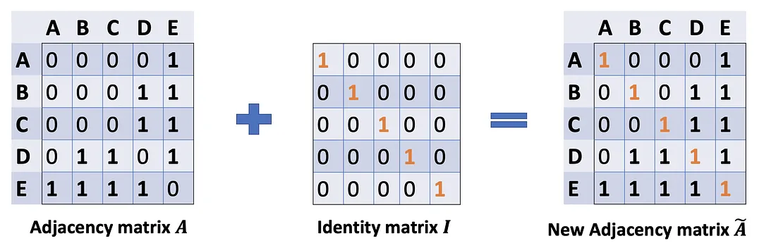
- We miss the feature of the node itself. For example, the first row of the result matrix should contain features of node A too.
- Instead of the sum() function, we need to take the average, or even better, the weighted average of neighbors’ feature vectors. Why don’t we use the sum() function? The reason is that when using the sum() function, high-degree nodes are likely to have huge v vectors, while low-degree nodes tend to get small aggregate vectors, which may later cause exploding or vanishing gradients (e.g., when using sigmoid). Besides, Neural networks seem to be sensitive to the scale of input data. Thus, we need to normalize these vectors to get rid of the potential issues.
In Problem (1), we can fix it by adding an Identity matrix I to A to get a new adjacency matrix Ã.
A ~ = A + λ I N \tilde{A}=A+\lambda I_N A~=A+λIN
Pick lambda = 1 (the feature of the node itself is just important as its neighbors), we have à = A + I. Note that we can treat lambda as a trainable parameter, but for now, just assign the lambda to 1, and even in the paper, lambda is just simply assigned to 1.
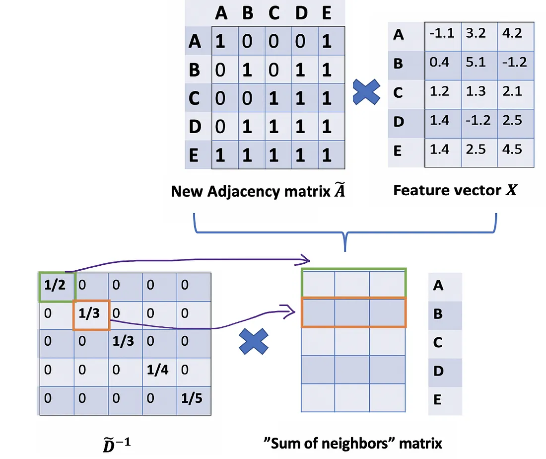
Problem (2): For matrix scaling, we usually multiply the matrix by a diagonal matrix. In this case, we want to take the average of the sum feature, or mathematically, to scale the sum vector matrix ÃX according to the node degrees. The gut feeling tells us that our diagonal matrix used to scale here is something related to the Degree matrix D̃ (Why D̃, not D? Because we’re considering Degree matrix D̃ of new adjacency matrix Ã, not A anymore).
The problem now becomes how we want to scale/normalize the sum vectors? In other words:
How we pass the information from neighbors to a specific node?
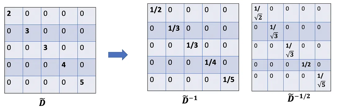
We would start with our old friend average. In this case, D̃ inverse (i.e., D̃^{-1}) comes into play. Basically, each element in D̃ inverse is the reciprocal of its corresponding term of the diagonal matrix D̃.

For example, node A has a degree of 2, so we multiple the sum vectors of node A by 1/2, while node E has a degree of 5, we should multiple the sum vector of E by 1/5, and so on.
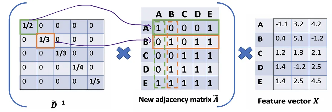
Thus, by taking the multiplication of D̃ inverse and X, we can take the average of all neighbors’ feature vectors (including itself).
So far so good. But you may ask How about the weighted average()?. Intuitively, it should be better if we treat high and low degree nodes differently.
Let’s take a deeper look at the average() approach that we’ve just mentioned. From the Associative property of matrix multiplication, for any three matrices A \mathrm{A} A, B \mathrm{B} B , and C \mathrm{C} C,( A B ) C = A ( B C \mathrm{A} B) \mathrm{C}=A(B \mathrm{C} AB)C=A(BC) . Rather D ~ − 1 ( A ~ X ) \tilde{D}^{-1}(\tilde{A} X) D~−1(A~X) , we consider ( D ~ − 1 A ~ ) X \left(\tilde{D}^{-1} \tilde{A}\right) X (D~−1A~)X , so D ~ − 1 \tilde{D}^{-1} D~−1 can also be seen as the scale factor of A ~ \tilde{A} A~ . From this perspective, each row i of A ~ \tilde{A} A~ will be scaled by D ~ i i \tilde{D}_{i i} D~ii (Figure below). Note that A ~ \tilde{A} A~ is a symmetric matrix, it means row i is the same value as column i . If we scale each row i by D ~ i i \tilde{D}_{i i} D~ii , intuitively, we have a feeling that we should do the same for its corresponding column too.
Mathematically, we’re scaling A ~ i j \tilde{A}_{i j} A~ij only by D ~ i i \tilde{D}_{i i} D~ii . We’re ignoring the j index. So, what would happen when we scale A ~ i j \tilde{A}_{i j} A~ij by both D ~ i i \tilde{D}_{i i} D~ii and D ~ j j \tilde{D}_{j j} D~jj ?
We try new scaling strategy: instead of using D ~ − 1 A ~ X \tilde{D}^{-1}\tilde{A}X D~−1A~X, we use D ~ − 1 A ~ D ~ − 1 X \tilde{D}^{-1}\tilde{A}\tilde{D}^{-1}X D~−1A~D~−1X.
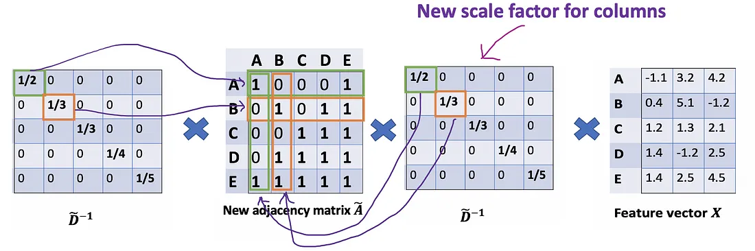
The new scaler gives us the “weighted” average. What we are doing here is to put more weights on the nodes that have low-degree and reduce the impact of high-degree nodes. The idea of this weighted average is that we assume low-degree nodes would have bigger impacts on their neighbors, whereas high-degree nodes generate lower impacts as they scatter their influence at too many neighbors.
One more minor note: When using two scalers( D ~ i i \tilde{D}_{ii} D~ii and D ~ j j \tilde{D}_{jj} D~jj ), we actually normalize twice, one time for the row as before, and another time for the column. It would make sense if we rebalance by modifying D ~ i i D ~ j j \tilde{D}_{ii}\tilde{D}_{jj} D~iiD~jj to D ~ i i D ~ j j \sqrt {\tilde{D}_{ii}\tilde{D}_{jj}} D~iiD~jj; ln other words, instead of using D ~ − 1 \tilde{D}^{-1} D~−1 , we use D ~ − 1 / 2 \tilde{D}^{-1/2} D~−1/2 .So,we further alter the formula to D ~ − 1 / 2 A ~ D ~ − 1 / 2 X \tilde{D}^{-1/2}\tilde{A}\tilde{D}^{-1/2}X D~−1/2A~D~−1/2X, which is exactly used in the paper.
Quick summary so far:
- A ~ X \tilde{A}X A~X: sum of all neighbors’ feature vectors, including itself.
- D ~ − 1 A ~ X : \tilde{D}^{-1}\tilde{A}X{:} D~−1A~X:averageof all eighbors’ feature vectors (including itself. Adjacency matrix is scaled by rows.
- D ~ − 1 / 2 A ~ D ~ − 1 / 2 X \tilde{D}^{-1/2}\tilde{A}\tilde{D}^{-1/2}X D~−1/2A~D~−1/2X: averageof all neighbors’ feature vectors (including itself). The adjacency matrix is scaled by both rows and columns. By doing this, we get the weighted average preferring on low-degree nodes.
Ok, now let’s put things together.
Let’s call A ^ = D ~ − 1 / 2 A ~ D ~ − 1 / 2 \hat{A}=\tilde{D}^{-1/2}\tilde{A}\tilde{D}^{-1/2} A^=D~−1/2A~D~−1/2 just for aclear view. With 2-layer GCN, we have the form of our forward mode as below.
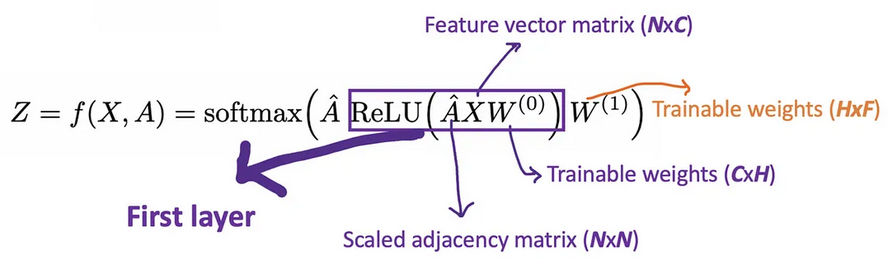
For example, we have a multi-classification problem with 10 classes, F will be set to 10. After having the 10-dimension vectors at layer 2, we pass these vectors through a softmax function for the prediction.
The Loss function is simply calculated by the cross-entropy error over all labeled examples, where Y_{l} is the set of node indices that have labels.
L = − ∑ l ∈ Y L ∑ f = 1 F Y l f ln Z l f \mathcal{L}=-\sum_{l\in\mathcal{Y}_L}\sum_{f=1}^FY_{lf}\ln Z_{lf} L=−l∈YL∑f=1∑FYlflnZlf
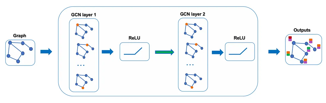
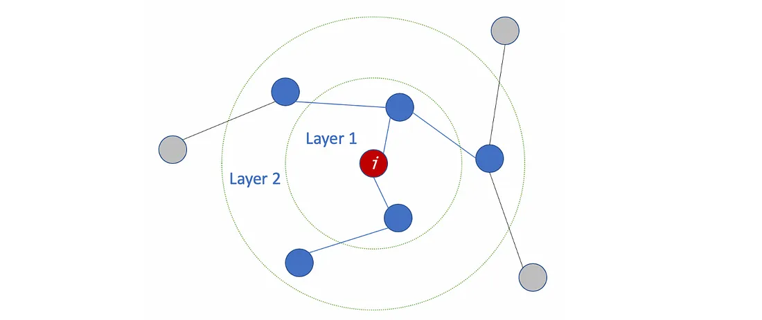
The number of layers
The meaning of #layers
The number of layers is the farthest distance that node features can travel. For example, with 1 layer GCN, each node can only get the information from its neighbors. The gathering information process takes place independently, at the same time for all the nodes.
When stacking another layer on top of the first one, we repeat the gathering info process, but this time, the neighbors already have information about their own neighbors (from the previous step). It makes the number of layers as the maximum number of hops that each node can travel. So, depends on how far we think a node should get information from the networks, we can config a proper number for #layers. But again, in the graph, normally we don’t want to go too far. With 6–7 hops, we almost get the entire graph, which makes the aggregation less meaningful.
How many layers should we stack the GCN?
In the paper, the authors also conducted some experiments with shallow and deep GCNs. From the figure below, we see that the best results are obtained with a 2- or 3-layer model. Besides, with a deep GCN (more than 7 layers), it tends to get bad performances (dashed blue line). One solution is to use the residual connections between hidden layers (purple line).
![Performance over #layers. Picture from the paper [3]](https://i-blog.csdnimg.cn/blog_migrate/7eb3dbb5a7a48a75b07ee61e4ffd75c0.png)
Take home notes
- GCNs are used for semi-supervised learning on the graph.
- GCNs use both node features and the structure for the training.
- The main idea of the GCN is to take the weighted average of all neighbors’ node features (including itself): Lower-degree nodes get larger weights. Then, we pass the resulting feature vectors through a neural network for training.
- We can stack more layers to make GCNs deeper. Consider residual connections for deep GCNs. Normally, we go for 2 or 3-layer GCN.
- Maths Note: When seeing a diagonal matrix, think of matrix scaling.
- A demo for GCN with StellarGraph library here [5]. The library also provides many other GNN algorithms. In addition, DGL [7] is another good library for GNNs. While StellarGraph helps us to set up the model easily, DGL aims to provide a more flexible structure which comes in handy when customizing our models.
Note from the authors of the paper.
The framework is currently limited to undirected graphs (weighted or unweighted). However, it is possible to handle both directed edges and edge features by representing the original directed graph as an undirected bipartite graph with additional nodes that represent edges in the original graph.
In the paper, the authors present the process from a Spectral perspective, while in this post, we go backward from the formula of GCN to understand how it handles the input graph from a Spatial point of view.
What’s next?
With GCNs, it seems we can make use of both the node features and the structure of the graph. However, what if the edges have different types? Should we treat each relationship differently? How to aggregate neighbors in this case? (R-GCN)
From another perspective, how can we further improve the GCN model? Is using fixed weights preferring on low-degree nodes good enough? Is there any way we can let the model learn the weights automatically by itself (Graph Attention Networks)? How can we deal with large graphs which can not be fitted in memory at once, or use more complex aggregators (GraphSAGE)?
In the next post on the graph topic, we will look into some more sophisticated GNN methods.
REFERENCES
[1] Excellent slides on Graph Representation Learning by Jure Leskovec (Stanford Course — cs224w): http://web.stanford.edu/class/cs224w/slides/07-noderepr.pdf
[2] Video Graph Convolutional Networks (GCNs) made simple: https://www.youtube.com/watch?v=2KRAOZIULzw
[3] Semi-supervised Classification with Graph Convolutional Networks (2017): https://arxiv.org/pdf/1609.02907.pdf
[4] GCN source code: https://github.com/tkipf/gcn
[5] Demo with StellarGraph library: https://stellargraph.readthedocs.io/en/stable/demos/node-classification/gcn-node-classification.html
[6] A Comprehensive Survey on Graph Neural Networks (2019): https://arxiv.org/pdf/1901.00596.pdf
[7] DGL Library: https://docs.dgl.ai/guide/graph.html


 3万+
3万+

 被折叠的 条评论
为什么被折叠?
被折叠的 条评论
为什么被折叠?
 到【灌水乐园】发言


