吴恩达Course1《神经网络与深度学习》week2:神经网络基础 测验及作业

第二周测验

1. 神经元节点先计算线性函数（z = Wx + b），再计算激活。注：神经元的输出是 a = g（Wx + b），其中 g 是激活函数（sigmoid，tanh，ReLU，…）

 2. 逻辑回归损失函数：𝐿(𝑦^(𝑖), 𝑦(𝑖)) = −𝑦(𝑖) log 𝑦^(𝑖)− (1 − 𝑦(𝑖))log(1 − 𝑦^(𝑖))

3. 假设 img 是一个（32,32,3）数组，具有 3 个颜色通道：红色、绿色和蓝色的 32x32 像素的图像。 如何将其重新转换为列向量？x = img.reshape((32 * 32 * 3, 1))

4.

a = np.random.randn(2, 3) # a.shape = (2, 3) 
b = np.random.randn(2, 1) # b.shape = (2, 1) 
c = a + b 

请问数组 c 的维度是多少？c.shape = (2, 3)

5. 

a = np.random.randn(4, 3) # a.shape = (4, 3)
b = np.random.randn(3, 2) # b.shape = (3, 2)
c = a * b

请问数组“c”的维度是多少？运算符 “*” 说明了按元素乘法来相乘，但是元素乘法需要两个矩阵之间的维数相同，所以这将报错，无法计算。计算矩阵乘法应使用np.dot(a,b)

6. 假设你的每一个样本有𝒏𝒙个输入特征，想一下在 𝑿 = [𝒙(𝟏), 𝒙(𝟐) … 𝒙(𝒎)] 中，X 的维度是多少？(𝑛𝑥, 𝑚)

7. 

a = np.random.randn(12288, 150) # a.shape = (12288, 150)
b = np.random.randn(150, 45) # b.shape = (150, 45)
c = np.dot(a, b)

 请问 c 的维度是多少？c.shape = (12288, 45)

8.

# a.shape = (3,4)
# b.shape = (4,1)
for i in range(3):
 for j in range(4):
 c[i][j] = a[i][j] + b[j]

请问要怎么把它们向量化？c = a + b.T

9. 

a = np.random.randn(3, 3)
b = np.random.randn(3, 1)
c = a * b

请问 c 的维度会是多少？ 这将会使用广播机制，b 会被复制三次，就会变成 (3,3)，再使用元素乘法。所以： c.shape = (3, 3)

10.

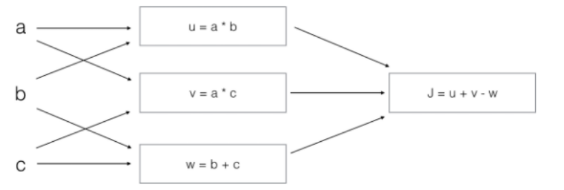问J输出什么？

J = u + v - w

= a * b + a * c - (b + c)

= a * (b + c) - (b + c)

= (a - 1) * (b + c)

第二周作业

Logistic Regression with a Neural Network mindset

欢迎来到您的第一个(必修课)编程作业!您将构建一个逻辑回归分类器来识别猫。这个作业将指导你如何用神经网络的心态来做这件事，因此也将磨练你关于深度学习的直觉。

产品说明:

• 不要在代码中使用循环(for/while)，除非指令明确要求这样做。

你将学会:

• 构建一个学习算法的总体架构，包括:
  • 初始化参数
  • 计算代价函数及其梯度
  • 使用一种优化算法(梯度下降)
• 按照正确的顺序将上面的三个函数聚集到一个主模型函数中。

1 - Packages

首先，让我们运行下面的单元格来导入在此任务期间需要的所有包。

• numpy是使用Python进行科学计算的基本包。
• h5py是一个通用包，用于与存储在H5文件中的数据集进行交互。
• matplotlib是Python中用于绘制图形的著名库。
• 这里用PIL和scipy来测试你的模型，最后用你自己的图片。

import numpy as np
import matplotlib.pyplot as plt
import h5py
import scipy
from PIL import Image
from scipy import ndimage
from lr_utils import load_dataset

%matplotlib inline

2 - Overview of the Problem set

问题陈述:你被给了一个数据集(“data.h5”)，包含:-一个m_train图像的训练集，标记为猫(y=1)或非猫(y=0) -一个m_test图像的测试集，标记为猫或非猫-每个图像的形状(num_px, num_px, 3)，其中

3是3个通道(RGB)。因此，每个图像都是正方形(高度= num_px)和正方形(宽度= num_px)。

您将构建一个简单的图像识别算法，可以正确地将图片分类为猫或非猫。

让我们更加熟悉数据集。通过运行以下代码加载数据。

# Loading the data (cat/non-cat)
train_set_x_orig, train_set_y, test_set_x_orig, test_set_y, classes = load_dataset()

我们在图像数据集(训练和测试)的末尾添加了“_trans”，因为我们要对它们进行预处理。预处理之后，我们将得到train_set_x和test_set_x(标签train_set_y和test_set_y不需要任何预处理)。

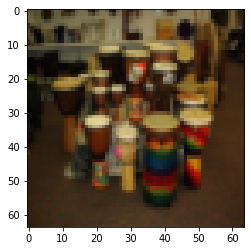
train_set_x_orig和test_set_x_orig的每一行都是一个表示图像的数组。您可以通过运行以下代码来可视化示例。您也可以随意更改索引值并重新运行以查看其他图像。

# Example of a picture
index = 5
plt.imshow(train_set_x_orig[index])
print ("y = " + str(train_set_y[:, index]) + ", it's a '" + classes[np.squeeze(train_set_y[:, index])].decode("utf-8") +  "' picture.")

y = [0], it's a 'non-cat' picture.

深度学习中的许多软件bug来自于矩阵/向量维度不匹配。如果你能保持矩阵/向量维数的平直，你就能在消除许多bug方面大有作为。

- m_train(训练示例的数量)- m_test(测试示例的数量)- num_px (= height =训练图像的宽度)记住train_set_x_orig是一个维度为(m_train, num_px, num_px, 3)的numpy数组。例如，你可以通过编写train_set_x_orig.shape[0]来访问m_train。

### START CODE HERE ### (≈ 3 lines of code)
m_train = train_set_x_orig.shape[0]
m_test = test_set_x_orig.shape[0]
num_px = train_set_x_orig.shape[1]

### END CODE HERE ###

print ("Number of training examples: m_train = " + str(m_train))
print ("Number of testing examples: m_test = " + str(m_test))
print ("Height/Width of each image: num_px = " + str(num_px))
print ("Each image is of size: (" + str(num_px) + ", " + str(num_px) + ", 3)")
print ("train_set_x shape: " + str(train_set_x_orig.shape))
print ("train_set_y shape: " + str(train_set_y.shape))
print ("test_set_x shape: " + str(test_set_x_orig.shape))
print ("test_set_y shape: " + str(test_set_y.shape))

Number of training examples: m_train = 209
Number of testing examples: m_test = 50
Height/Width of each image: num_px = 64
Each image is of size: (64, 64, 3)
train_set_x shape: (209, 64, 64, 3)
train_set_y shape: (1, 209)
test_set_x shape: (50, 64, 64, 3)
test_set_y shape: (1, 50)

Expected Output for m_train, m_test and num_px:

**m_train**	209
**m_test**	50
**num_px**	64

为了方便，现在应该在numpy数组(num_px * num_px * 3,1)中重塑维度(num_px, num_px, 3)的图像。在此之后，我们的训练(和测试)数据集是一个numpy数组，其中每一列表示一个扁平图像。应该有m_train(分别是m_test)列。

重塑训练和测试数据集，使大小(num_px, num_px, 3)的图像被平展成单个形状向量(num_px * num_px * 3,1)。

当你想要将形状矩阵X (A,b,c,d)平化为形状矩阵X_flatten (b∗c∗d, A)时，有一个技巧要使用:

X_flatten = X.reshape(X.shape[0], -1).T      # X.T is the transpose of X

# Reshape the training and test examples

### START CODE HERE ### (≈ 2 lines of code)
train_set_x_flatten = train_set_x_orig.reshape(train_set_x_orig.shape[0], -1).T
test_set_x_flatten = test_set_x_orig.reshape(test_set_x_orig.shape[0], -1).T

### END CODE HERE ###

print ("train_set_x_flatten shape: " + str(train_set_x_flatten.shape))
print ("train_set_y shape: " + str(train_set_y.shape))
print ("test_set_x_flatten shape: " + str(test_set_x_flatten.shape))
print ("test_set_y shape: " + str(test_set_y.shape))
print ("sanity check after reshaping: " + str(train_set_x_flatten[0:5,0]))

Expected Output:

**train_set_x_flatten shape**	(12288, 209)
**train_set_y shape**	(1, 209)
**test_set_x_flatten shape**	(12288, 50)
**test_set_y shape**	(1, 50)
**sanity check after reshaping**	[17 31 56 22 33]

为了表示彩色图像，必须为每个像素指定红、绿和蓝通道(RGB)，因此像素值实际上是一个由0到255三个数字组成的向量。

机器学习中一个常见的预处理步骤是集中并标准化数据集，这意味着从每个示例中减去整个numpy数组的平均值，然后将每个示例除以整个numpy数组的标准差。但是对于图片数据集，将数据集的每一行除以255(像素通道的最大值)就更简单、更方便了。

让我们标准化数据集。

train_set_x = train_set_x_flatten/255.
test_set_x = test_set_x_flatten/255.

你需要记住的是:

预处理新数据集的常见步骤如下:

• 找出问题的尺寸和形状(m_train, m_test, num_px，…)
• 重塑数据集，使每个示例现在都是一个大小向量(num_px * num_px * 3,1)
• “标准化”的数据

 3 - General Architecture of the learning algorithm

现在是时候设计一个简单的算法来区分猫图像和非猫图像了。

你将建立一个逻辑回归，使用神经网络思维。下图解释了为什么逻辑回归实际上是一个非常简单的神经网络!

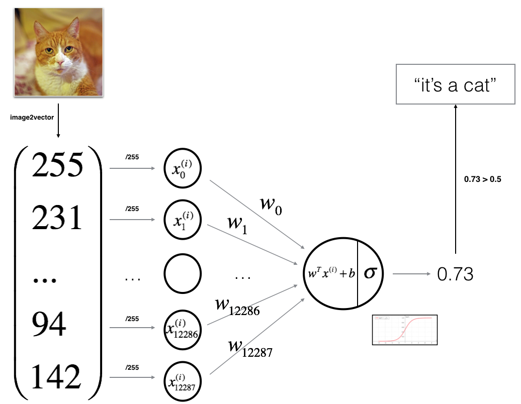
Mathematical expression of the algorithm:

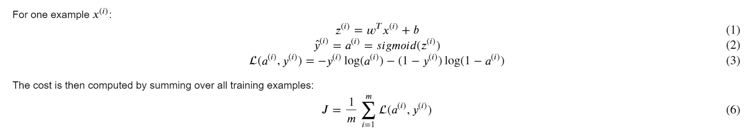
关键步骤:在本练习中，您将执行以下步骤:—初始化模型参数—通过最小化成本来学习模型参数

-使用学习到的参数进行预测(在测试集上)-分析结果并得出结论

 4 - Building the parts of our algorithm

构建神经网络的主要步骤是:

建立神经网络的主要步骤是：

1. 定义模型结构（例如输入特征的数量）

2. 初始化模型的参数

3. 循环：

   3.1 计算当前损失（正向传播）

   3.2 计算当前梯度（反向传播）

   3.3 更新参数（梯度下降）

分别构建上述1-3，并将它们集成到一个函数中，我们称之为model()。

4.1 -辅助功能

使用“Python基础”中的代码，实现sigmoid()。正如您所看到的在上面的图中,需要计算进行预测。，使用np.exp()。

# GRADED FUNCTION: sigmoid

def sigmoid(z):
    """
    Compute the sigmoid of z

    Arguments:
    z -- A scalar or numpy array of any size.

    Return:
    s -- sigmoid(z)
    """

    ### START CODE HERE ### (≈ 1 line of code)
    s = 1 / (1 + np.exp(-z))
    ### END CODE HERE ###
    
    return s

print ("sigmoid([0, 2]) = " + str(sigmoid(np.array([0,2]))))

Expected Output:

**sigmoid([0, 2])**

[ 0.5 0.88079708]

4.2 -初始化参数

在下面的单元格中实现参数初始化。你必须把w初始化为一个零向量。如果您不知道要使用什么numpy函数，请在numpy库的文档中查找np.zeros()。

# GRADED FUNCTION: initialize_with_zeros

def initialize_with_zeros(dim):
    """
    This function creates a vector of zeros of shape (dim, 1) for w and initializes b to 0.
    
    Argument:
    dim -- size of the w vector we want (or number of parameters in this case)
    
    Returns:
    w -- initialized vector of shape (dim, 1)
    b -- initialized scalar (corresponds to the bias)
    """
    
    ### START CODE HERE ### (≈ 1 line of code)
    w = np.zeros((dim, 1))
    b = 0
    ### END CODE HERE ###

    assert(w.shape == (dim, 1))
    assert(isinstance(b, float) or isinstance(b, int))
    
    return w, b

dim = 2
w, b = initialize_with_zeros(dim)
print ("w = " + str(w))
print ("b = " + str(b))

Expected Output:

** w **	[[ 0.] [ 0.]]
** b **	0

For image inputs, w will be of shape (num_px * num_px * 3, 1).

4.3 -向前和向后传播

现在已经初始化了参数，您可以执行“向前”和“向后”传播步骤来学习参数。

实现一个propagate()函数，该函数计算代价函数及其梯度。

提示:

# GRADED FUNCTION: propagate

def propagate(w, b, X, Y):
    """
    Implement the cost function and its gradient for the propagation explained above

    Arguments:
    w -- weights, a numpy array of size (num_px * num_px * 3, 1)
    b -- bias, a scalar
    X -- data of size (num_px * num_px * 3, number of examples)
    Y -- true "label" vector (containing 0 if non-cat, 1 if cat) of size (1, number of examples)

    Return:
    cost -- negative log-likelihood cost for logistic regression
    dw -- gradient of the loss with respect to w, thus same shape as w
    db -- gradient of the loss with respect to b, thus same shape as b
    
    Tips:
    - Write your code step by step for the propagation. np.log(), np.dot()
    """
    
    m = X.shape[1]
    
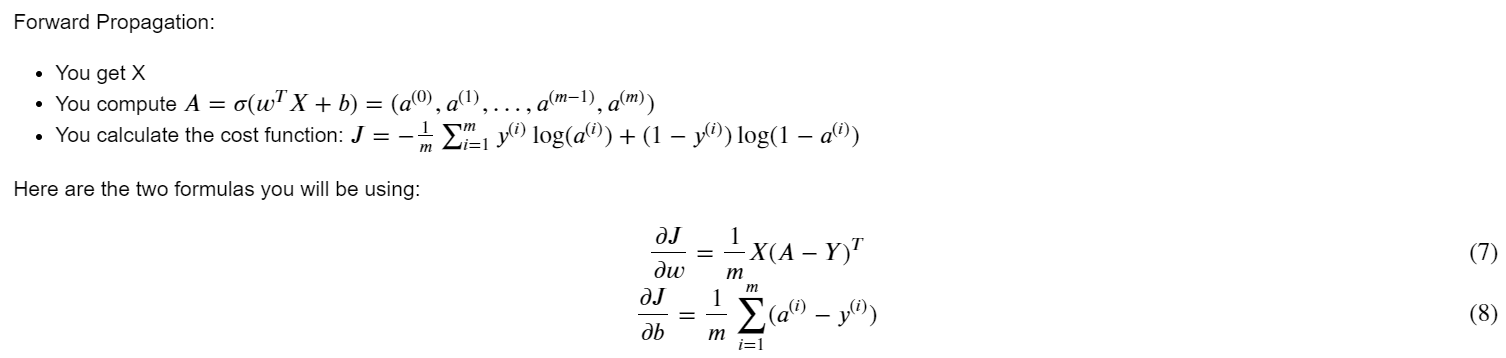
    # FORWARD PROPAGATION (FROM X TO COST)
    ### START CODE HERE ### (≈ 2 lines of code)
    Z = np.dot(w.T, X) + b
    A = sigmoid(Z)
    cost = 1/m * np.sum(-Y*np.log(A)-(1-Y)*np.log(1-A))
    ### END CODE HERE ###
    
    # BACKWARD PROPAGATION (TO FIND GRAD)
    ### START CODE HERE ### (≈ 2 lines of code)
    dZ = A - Y
    dw = 1/m * np.dot(X, dZ.T)
    db = 1/m * np.sum(dZ)
    ### END CODE HERE ###
    assert(dw.shape == w.shape)
    assert(db.dtype == float)
    cost = np.squeeze(cost)
    assert(cost.shape == ())
    
    grads = {"dw": dw,
             "db": db}
    
    return grads, cost

w, b, X, Y = np.array([[1],[2]]), 2, np.array([[1,2],[3,4]]), np.array([[1,0]])
grads, cost = propagate(w, b, X, Y)
print ("dw = " + str(grads["dw"]))
print ("db = " + str(grads["db"]))
print ("cost = " + str(cost))

Expected Output:

** dw **	[[ 0.99993216] [ 1.99980262]]
** db **	0.499935230625
** cost **	6.000064773192205

d)优化

• 您已经初始化了参数。
• 你也可以计算一个代价函数和它的梯度。
• 现在，您希望使用梯度下降来更新参数。

练习:写出优化函数。目标是通过最小化成本函数𝐽来学习𝑤和𝑏。对于𝜃，更新规则为𝜃=𝜃−𝛼𝑑𝜃，其中𝛼为学习率。

params, grads, costs = optimize(w, b, X, Y, num_iterations= 100, learning_rate = 0.009, print_cost = False)

print ("w = " + str(params["w"]))
print ("b = " + str(params["b"]))
print ("dw = " + str(grads["dw"]))
print ("db = " + str(grads["db"]))
print(costs)

w = [[0.1124579 ]
 [0.23106775]]
b = 1.5593049248448891
dw = [[0.90158428]
 [1.76250842]]
db = 0.4304620716786828
[6.000064773192205]

前面的函数将输出学习到的w和b。我们可以使用w和b来预测数据集x的标签。计算预测有两个步骤:

• 计算𝑌̂=𝐴=𝜎(𝑤𝑇𝑋+𝑏)
• 将a的条目转换为0(如果激活<= 0.5)或1(如果激活> 0.5)，将预测存储在Y_prediction向量中。如果您愿意，您可以在for循环中使用If /else语句(尽管也有一种方法对其进行向量化)。

# GRADED FUNCTION: predict

def predict(w, b, X):
    '''
    Predict whether the label is 0 or 1 using learned logistic regression parameters (w, b)
    
    Arguments:
    w -- weights, a numpy array of size (num_px * num_px * 3, 1)
    b -- bias, a scalar
    X -- data of size (num_px * num_px * 3, number of examples)
    
    Returns:
    Y_prediction -- a numpy array (vector) containing all predictions (0/1) for the examples in X
    '''
    
    m = X.shape[1]
    Y_prediction = np.zeros((1,m))
    w = w.reshape(X.shape[0], 1)
    
    # Compute vector "A" predicting the probabilities of a cat being present in the picture
    ### START CODE HERE ### (≈ 1 line of code)
    A = sigmoid(np.dot(w.T, X) + b)
    ### END CODE HERE ###

    for i in range(A.shape[1]):
        
        # Convert probabilities A[0,i] to actual predictions p[0,i]
        ### START CODE HERE ### (≈ 4 lines of code)
        Y_prediction[0,i] = 1 if A[0,i] > 0.5 else 0
        ### END CODE HERE ###
    
    assert(Y_prediction.shape == (1, m))
    
    return Y_prediction

print ("predictions = " + str(predict(w, b, X)))

Expected Output:

**predictions**

[[ 1. 1.]]

记住:你已经实现了几个函数:-初始化(w,b) -优化损失迭代学习参数(w,b): -计算成本和其梯度-使用梯度下降更新参数-使用学习(w,b)预测标签为给定的一组示例 

5 - Merge all functions into a model

现在，您将看到如何通过将所有构建块(前面部分中实现的函数)以正确的顺序组合在一起来构建整个模型。

实现模型函数。使用以下符号:—Y_prediction用于测试集上的预测—Y_prediction_train用于训练集上的预测—w、成本、梯度用于optimize()的输出

# GRADED FUNCTION: model

def model(X_train, Y_train, X_test, Y_test, num_iterations = 2000, learning_rate = 0.5, print_cost = False):
    """
    Builds the logistic regression model by calling the function you've implemented previously
    
    Arguments:
    X_train -- training set represented by a numpy array of shape (num_px * num_px * 3, m_train)
    Y_train -- training labels represented by a numpy array (vector) of shape (1, m_train)
    X_test -- test set represented by a numpy array of shape (num_px * num_px * 3, m_test)
    Y_test -- test labels represented by a numpy array (vector) of shape (1, m_test)
    num_iterations -- hyperparameter representing the number of iterations to optimize the parameters
    learning_rate -- hyperparameter representing the learning rate used in the update rule of optimize()
    print_cost -- Set to true to print the cost every 100 iterations
    
    Returns:
    d -- dictionary containing information about the model.
    """
    
    ### START CODE HERE ###
    
    # initialize parameters with zeros (≈ 1 line of code)
    w , b = initialize_with_zeros(X_train.shape[0])
    
    # Gradient descent (≈ 1 line of code)
    parameters , grads , costs = optimize(w , b , X_train , Y_train, num_iterations , learning_rate , print_cost)
    
    # Retrieve parameters w and b from dictionary "parameters"
    w , b = parameters["w"] , parameters["b"]
    
    # Predict test/train set examples (≈ 2 lines of code)
    Y_prediction_test = predict(w , b, X_test)
    Y_prediction_train = predict(w , b, X_train)
    
    ### END CODE HERE ###

    # Print train/test Errors
    print("train accuracy: {} %".format(100 - np.mean(np.abs(Y_prediction_train - Y_train)) * 100))
    print("test accuracy: {} %".format(100 - np.mean(np.abs(Y_prediction_test - Y_test)) * 100))

    
    d = {"costs": costs,
         "Y_prediction_test": Y_prediction_test, 
         "Y_prediction_train" : Y_prediction_train, 
         "w" : w, 
         "b" : b,
         "learning_rate" : learning_rate,
         "num_iterations": num_iterations}
    
    return d

d = model(train_set_x, train_set_y, test_set_x, test_set_y, num_iterations = 2000, learning_rate = 0.005, print_cost = True)

Cost after iteration 0: 0.693147
Cost after iteration 100: 0.584508
Cost after iteration 200: 0.466949
Cost after iteration 300: 0.376007
Cost after iteration 400: 0.331463
Cost after iteration 500: 0.303273
Cost after iteration 600: 0.279880
Cost after iteration 700: 0.260042
Cost after iteration 800: 0.242941
Cost after iteration 900: 0.228004
Cost after iteration 1000: 0.214820
Cost after iteration 1100: 0.203078
Cost after iteration 1200: 0.192544
Cost after iteration 1300: 0.183033
Cost after iteration 1400: 0.174399
Cost after iteration 1500: 0.166521
Cost after iteration 1600: 0.159305
Cost after iteration 1700: 0.152667
Cost after iteration 1800: 0.146542
Cost after iteration 1900: 0.140872
train accuracy: 99.04306220095694 %
test accuracy: 70.0 %

点评:训练准确率接近100%。这是一个很好的完整性检查:您的模型正在工作，并且具有足够高的容量来拟合训练数据。测试误差为68%。对于这个简单的模型来说，它实际上并不坏，因为我们使用的数据集很小，而且逻辑回归是一个线性分类器。但不用担心，下周您将构建一个更好的分类器!

此外，您可以看到，该模型显然对训练数据进行了过拟合。在本专题的后面，您将学习如何减少过拟合，例如使用正则化。使用下面的代码(并更改索引变量)，您可以查看测试集图片上的预测。

# Plot learning curve (with costs)
costs = np.squeeze(d['costs'])
plt.plot(costs)
plt.ylabel('cost')
plt.xlabel('iterations (per hundreds)')
plt.title("Learning rate =" + str(d["learning_rate"]))
plt.show()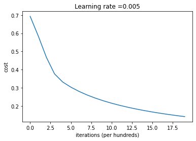

解读:你可以看到成本在下降。这表明参数正在被学习。但是，您可以看到，您可以在训练集中对模型进行更多的训练。尝试增加上面单元格中的迭代次数，并重新运行单元格。你可能会发现训练集的准确率上升了，但测试集的准确率下降了。这叫做过拟合。

6 - Further analysis (optional/ungraded exercise)

祝贺您建立了第一个图像分类模型。让我们进一步分析它，并检查学习率𝛼的可能选择。 

学习速率的选择：

提醒:为了让梯度下降发挥作用，你必须明智地选择学习率。学习率𝛼决定了我们更新参数的速度。如果学习率太大，我们可能会“超过”最优值。类似地，如果它太小，我们将需要太多的迭代才能收敛到最佳值。这就是为什么使用一个良好的学习率是至关重要的。

让我们将模型的学习曲线与几种学习率的选择进行比较。运行下面的单元格。这个过程大约需要1分钟。您也可以尝试不同的值，而不是我们初始化的learning_rates变量所包含的三个值，看看会发生什么。

learning_rates = [0.01, 0.001, 0.0001]
models = {}
for i in learning_rates:
    print ("learning rate is: " + str(i))
    models[str(i)] = model(train_set_x, train_set_y, test_set_x, test_set_y, num_iterations = 1500, learning_rate = i, print_cost = False)
    print ('\n' + "-------------------------------------------------------" + '\n')

for i in learning_rates:
    plt.plot(np.squeeze(models[str(i)]["costs"]), label= str(models[str(i)]["learning_rate"]))

plt.ylabel('cost')
plt.xlabel('iterations')

legend = plt.legend(loc='upper center', shadow=True)
frame = legend.get_frame()
frame.set_facecolor('0.90')
plt.show()

learning rate is: 0.01
train accuracy: 99.52153110047847 %
test accuracy: 68.0 %

-------------------------------------------------------

learning rate is: 0.001
train accuracy: 88.99521531100478 %
test accuracy: 64.0 %

-------------------------------------------------------

learning rate is: 0.0001
train accuracy: 68.42105263157895 %
test accuracy: 36.0 %

-------------------------------------------------------

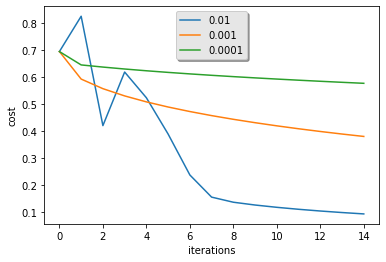
解释:

• 不同的学习率会带来不同的成本，从而导致不同的预测结果。
• 如果学习率太大(0.01)，代价可能会上下振荡。它甚至可能会产生分歧(尽管在本例中，使用0.01最终仍然会获得较好的成本值)。
• 更低的成本并不意味着更好的模式。你必须检查是否有可能过度拟合。当训练的准确度远远高于测试的准确度时，就会出现这种情况。
• 在深度学习中，我们通常推荐你:
  •  选择能使代价函数最小的学习率。
  •  如果你的模型过度拟合，使用其他技术来减少过度拟合。(我们会在后面的视频中讲到)

逻辑回归关键代码

# 导入包
import numpy as np
import matplotlib.pyplot as plt

"""
    计算z的sigmoid函数
    参数:
    z -- 任何大小的标量或numpy数组
    返回:
    s -- sigmoid(z)
"""
def sigmoid(z):
 
    s = 1 / (1 + np.exp(-z))
    
    return s

"""
    此函数为w创建一个维度为（dim，1）的0向量，并将b初始化为0。
        
    参数：
        dim  - 我们想要的w矢量的大小（或者这种情况下的参数数量）
        
    返回：
        w  - 维度为（dim，1）的初始化向量。
        b  - 初始化的标量（对应于偏差）
"""
def initialize_with_zeros(dim):
    
    w = np.zeros(shape = (dim,1))
    b = 0
    #使用断言来确保我要的数据是正确的
    assert(w.shape == (dim, 1)) #w的维度是(dim,1)
    assert(isinstance(b, float) or isinstance(b, int)) #b的类型是float或者是int
    
    return (w , b)

"""
    实现前向和后向传播的成本函数及其梯度。
    参数：
        w  - 权重，大小不等的数组（num_px * num_px * 3，1）
        b  - 偏差，一个标量
        X  - 矩阵类型为（num_px * num_px * 3，训练数量）
        Y  - 真正的“标签”矢量（如果非猫则为0，如果是猫则为1），矩阵维度为(1,训练数据数量)

    返回：
        cost- 逻辑回归的负对数似然成本
        dw  - 相对于w的损失梯度，因此与w相同的形状
        db  - 相对于b的损失梯度，因此与b的形状相同
"""
def propagate(w, b, X, Y):
    m = X.shape[1]
    
    #正向传播
    A = sigmoid(np.dot(w.T,X) + b) 
    cost = (- 1 / m) * np.sum(Y * np.log(A) + (1 - Y) * (np.log(1 - A))) 
    
    #反向传播
    dw = (1 / m) * np.dot(X, (A - Y).T) 
    db = (1 / m) * np.sum(A - Y) 

    #使用断言确保我的数据是正确的
    assert(dw.shape == w.shape)
    assert(db.dtype == float)
    cost = np.squeeze(cost)
    assert(cost.shape == ())
    
    #创建一个字典，把dw和db保存起来。
    grads = {
                "dw": dw,
                "db": db
             }
    return (grads , cost)

"""
    此函数通过运行梯度下降算法来优化w和b
    
    参数：
        w  - 权重，大小不等的数组（num_px * num_px * 3，1）
        b  - 偏差，一个标量
        X  - 维度为（num_px * num_px * 3，训练数据的数量）的数组。
        Y  - 真正的“标签”矢量（如果非猫则为0，如果是猫则为1），矩阵维度为(1,训练数据的数量)
        num_iterations  - 优化循环的迭代次数
        learning_rate  - 梯度下降更新规则的学习率
        print_cost  - 每100步打印一次损失值
    
    返回：
        params  - 包含权重w和偏差b的字典
        grads  - 包含权重和偏差相对于成本函数的梯度的字典
        成本 - 优化期间计算的所有成本列表，将用于绘制学习曲线。
    
    提示：
    我们需要写下两个步骤并遍历它们：
        1）计算当前参数的成本和梯度，使用propagate（）。
        2）使用w和b的梯度下降法则更新参数。
"""
def optimize(w , b , X , Y , num_iterations , learning_rate , print_cost = False):
    
    costs = []
    
    for i in range(num_iterations):
        
        grads, cost = propagate(w, b, X, Y)
        
        dw = grads["dw"]
        db = grads["db"]
        
        w = w - learning_rate * dw
        b = b - learning_rate * db
        
        #记录成本 每迭代100次记录一次
        if i % 100 == 0:
            costs.append(cost)
        #打印成本数据
        if (print_cost) and (i % 100 == 0):
            print("迭代的次数: %i ， 误差值： %f" % (i,cost))
        
    params  = {
                "w" : w,
                "b" : b }
    grads = {
            "dw": dw,
            "db": db } 
    return (params , grads , costs)

"""
    使用学习逻辑回归参数logistic （w，b）预测标签是0还是1，
    
    参数：
        w  - 权重，大小不等的数组（num_px * num_px * 3，1）
        b  - 偏差，一个标量
        X  - 维度为（num_px * num_px * 3，训练数据的数量）的数据
    
    返回：
        Y_prediction  - 包含X中所有图片的所有预测【0 | 1】的一个numpy数组（向量）
    
"""
def predict(w , b , X ):
    
    m  = X.shape[1] #样本的数量
    Y_prediction = np.zeros((1,m)) 
    w = w.reshape(X.shape[0],1)
    
    #计预测猫在图片中出现的概率
    A = sigmoid(np.dot(w.T , X) + b)
    for i in range(A.shape[1]):
        #将概率a [0，i]转换为实际预测p [0，i]
        Y_prediction[0,i] = 1 if A[0,i] > 0.5 else 0
    #使用断言
    assert(Y_prediction.shape == (1,m))
    
    return Y_prediction

"""
    通过调用之前实现的函数来构建逻辑回归模型
    
    参数：
        X_train  - numpy的数组,维度为（num_px * num_px * 3，m_train）的训练集
        Y_train  - numpy的数组,维度为（1，m_train）（矢量）的训练标签集
        X_test   - numpy的数组,维度为（num_px * num_px * 3，m_test）的测试集
        Y_test   - numpy的数组,维度为（1，m_test）的（向量）的测试标签集
        num_iterations  - 表示用于优化参数的迭代次数的超参数
        learning_rate  - 表示optimize（）更新规则中使用的学习速率的超参数
        print_cost  - 设置为true以每100次迭代打印成本
    
    返回：
        d  - 包含有关模型信息的字典。
"""
def model(X_train , Y_train , X_test , Y_test , num_iterations = 2000 , learning_rate = 0.5 , print_cost = False):
    
    w , b = initialize_with_zeros(X_train.shape[0])
    
    parameters , grads , costs = optimize(w , b , X_train , Y_train, num_iterations , learning_rate , print_cost)
    
    #从字典“参数”中检索参数w和b
    w , b = parameters["w"] , parameters["b"]
    
    #预测测试/训练集的例子
    Y_prediction_test = predict(w , b, X_test)
    Y_prediction_train = predict(w , b, X_train)
    
    #打印训练后的准确性
    print("训练集准确性："  , format(100 - np.mean(np.abs(Y_prediction_train - Y_train)) * 100) ,"%")
    print("测试集准确性："  , format(100 - np.mean(np.abs(Y_prediction_test - Y_test)) * 100) ,"%")
    
    d = {
            "costs" : costs,
            "Y_prediction_test" : Y_prediction_test,
            "Y_prediciton_train" : Y_prediction_train,
            "w" : w,
            "b" : b,
            "learning_rate" : learning_rate,
            "num_iterations" : num_iterations 
        }
    return d