


 文章介绍了基于LMDB电影影评数据集进行情感分类的方法,包括数据预处理(构造词频表,去除特殊符号和停用词)、特征工程(使用积极和消极词汇的词频和TF/TDF交叉熵)以及使用支持向量机、逻辑回归和K近邻三种机器学习算法进行模型训练,结果显示支持向量机表现最佳。
基于LMDB电影影评数据集进行情感分类
数据集介绍
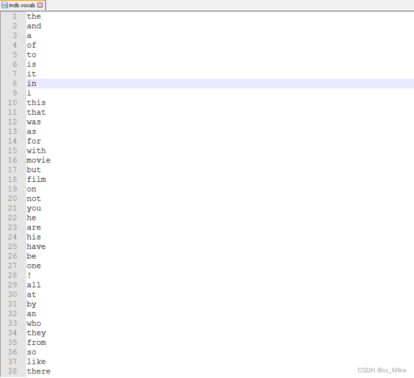
标签数据集包含5万条IMDB影评,专门用于情绪分析。评论的情绪是二元的,这意味着IMDB评级< 5导致情绪得分为0,而评级>=7的情绪得分为1。没有哪部电影的评论超过30条。标有training set的2.5万篇影评不包括与2.5万篇影评测试集相同的电影。此外,还有另外5万篇IMDB影评没有任何评级标签。其中lmdb有已构建好的词表imdb.vocab 字典囊括了数据集中出现的词,词在字典中的位置按照词在数据集中出现的次数从大到小排列,这个字典大小为89527。这里可以直接使用字典进行特征工程和训练,当然你也可以自己构造字典进行标注更多的信息,为特征工程提供便捷。
本篇文章将介绍如何构造词典,并通过词典进行构造特征工程训练完成评论情感的二分类。

数据预处理:词频表的构造
要完成对文字情感分类,首先需要清楚评论中是否包含褒贬词汇,当一篇评论中贬义词汇较多时,我们会更加倾向于认为它是一个消极的评论。那么基于此,我们首先需要根据训练数据集褒贬评论来构造褒贬词典。本篇文章设计的词典结构不按照出现次数排序,而直接记录每个词出现的频数,这么做是为了便于后期特征工程时分辨褒贬词频(因为不依靠该数据集之外的词典,直接通过褒义评论构造褒义词频表,贬义词汇构造贬义词频表,其所构造的词表中可能存在中性词或未被筛除的停用词从而造成情感文本分类不准确)工作,提高特征工程对文本分类的质量。在此分类工作的主要流程如下图所示:
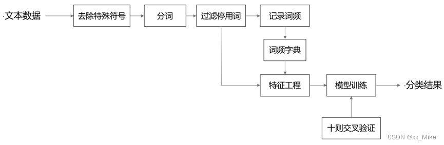
从上图可以看出,分类工作分成两步,构造词频表和特征工程模型训练,在构造词频字典时,遍历所有文本,对每个评论文本分别需要进行去除特殊符号,分词,过滤停用词的操作。
去除特殊符号与分词:每个文本中包含除字符外的其它标符,如“()<>,.!”等等,这些符号若不进行清理,会污染所构造的词典,从而对分类产生影响。当然去除这些符号我们可以直接通过正则表达式进行替换即可,如下所示:通过re模块进行特殊符号的清除,通过将空格标记进行分词分别完成去除符号与分词操作,得到评论的词汇表vocabList。当然在此需要注意的一点是,清除逗号句号等标记符时需要将其替换为空格而不是直接去除,防止在分词时将两个词记为一个词。
 print("开始第{}批词语处理进入语料库,当前语料库共有{}个词汇".format(count, len(vocabf_dict)))
            vocabList = re.sub("\<.*?\>", '', vocabList)
            vocabList = re.sub("\[.*?\]", '', vocabList)
            vocabList = re.sub('[0-9’!"#$%&\'()*+,-./:;<=>?@,。?★、…【】《》?“”‘’![\\]^_`{|}~]+','',vocabList)
            vocabList = vocabList.replace(",", " ").replace(".", " ").replace("'", " ").replace('"', " ").split()
去除停用词汇:在此停用词汇主要指的是如冠词等对情感分类无作用的词汇,如:"the,a,I,I’m"等等,这个停用词汇表可在网上获取,当然停用词汇越充分,其能剔除掉的无用词汇就越多,对文本分类将更有利,本文所使用的停用词表共891个词(附资源处供下载),即分词列表中需要剔除掉处于停用词表中的词。
完成上述预处理后,就能进行词频统计,遍历完所有评论即可完成词频表的构造啦,在此将词频表保存为pkl格式待特征工程使用。
下面为构造词频表的函数:
'''生成词频表'''
    def create_vocabf(self,config):
        vocabf_dict = {}
        vocabf_dict_num = 0
        loadPath = config.path
        runBatch = config.runBatch
        textNum = 0
        vocabList = ""
        count = 1
        sumCount = 1
        textNameList = os.listdir(loadPath)
        for textName in textNameList:
            loadPathCash = loadPath +  "/" + textName
            if textNum != len(textNameList):
                if (textNum % runBatch != 0 or textNum == 0):
                    with open(loadPathCash, encoding="utf-8") as f:
                        vocabList = vocabList + " " + f.read().lower()
                    textNum = textNum + 1
                    sumCount = sumCount + 1
                    continue
            # 去除符号,括号,以及停用词汇
            print("开始第{}批词语处理进入语料库,当前语料库共有{}个词汇".format(count, len(vocabf_dict)))
            vocabList = re.sub("\<.*?\>", '', vocabList)
            vocabList = re.sub("\(.*?\)", '', vocabList)
            vocabList = re.sub("\[.*?\]", '', vocabList)
            vocabList = re.sub('[0-9’!"#$%&\'()*+,-./:;<=>?@,。?★、…【】《》?“”‘’![\\]^_`{|}~]+','',vocabList)
            vocabList = vocabList.replace(",", " ").replace(".", " ").replace("'", " ").replace('"', " ").split()
            for vocab in vocabList:
                # 过滤停用词
                if vocab not in self.stopWords:
                    # 不在字典则添加,否则增加频数
                    if vocab not in vocabf_dict.keys():
                        vocabf_dict[vocab] = 1
                        vocabf_dict_num = vocabf_dict_num + 1
                    else:
                        vocabf_dict[vocab] = vocabf_dict[vocab] + 1

            vocabList = ""
            count = count + 1
            textNum = 0
        dict_save = open(config.saveName + '.pkl', 'wb')
        pickle.dump(vocabf_dict, dict_save)
根据上述方法分别构造出褒义词频表和贬义词频表为后期特征工程及训练做准备,如下图所示。

特征工程
由于本文采用机器学习算法进行模型训练,故特征工程的建立是非常重要且必不可少的,感兴趣的朋友也可以通过构造好的词频表尝试进行神经网络训练(不需要特征工程的步骤),在该工作过程中,由于特征的选取认为因素较大,故特征的选取对后期文本分类影响也较大,这里本文共提出4个特征来对其进行训练。特征描述如下:
1. 文本积极词汇出现次数num_pos
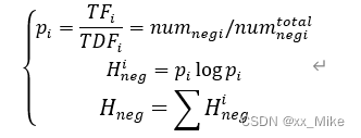
2. 文本消极词汇出现次数num_neg
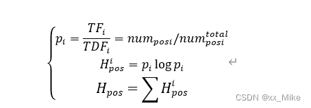
3. 文本积极词汇TF/TDF的交叉熵H_pos
特征工程生成代码如下:
'''文本读取:生成np矩阵,特征选取:1 积极性词汇出现总数 2 消极性词汇出现总数 3 积极性词汇信息熵 4 消极性词汇信息熵'''
    def textBatchLoad(self,config , choose):
        featureInput = []
        if choose:
            textLoadPath = config.posPath
        else:
            textLoadPath = config.negPath
        textNameList = os.listdir(textLoadPath)
        f_read = open(config.posVocabfPath, 'rb')
        posDict = pickle.load(f_read)
        f_read = open(config.negVocabfPath, 'rb')
        negDict = pickle.load(f_read)
        f_read.close()
        count = 0
        for text in textNameList:
            if count % 50 == 0:
                print("开始处理第{}个文本".format(count))
            with open(textLoadPath + '/' + text, encoding= 'gbk' ,errors= 'ignore') as f:
                vocabList = f.read().lower()
                vocabList = re.sub("\<.*?\>", '', vocabList)
                vocabList = re.sub("\(.*?\)", '', vocabList)
                vocabList = re.sub("\[.*?\]", '', vocabList)
                vocabList = vocabList.replace(",", " ").replace(".", " ").replace("'", " ").replace('"', " ")
                vocabList = re.sub('[0-9’!"#$%&\'()*+,-./:;<=>?@,。?★、…【】《》?“”‘’![\\]^_`{|}~]+', '', vocabList).split()
            posCount = 0
            negCount = 0
            posCross = 0
            negCross = 0
            cashList = []
            featureInputCash = []
            for vocab in vocabList:
                if vocab not in cashList:
                    if vocab in posDict:
                        posCount = posCount + vocabList.count(vocab)
                        posCross = posCross + \
                                   (vocabList.count(vocab)/posDict[vocab])*np.log((vocabList.count(vocab)/posDict[vocab]))
                    if vocab in negDict:
                        negCount = negCount + vocabList.count(vocab)
                        negCross = negCross + \
                                   (vocabList.count(vocab) / negDict[vocab]) * np.log((vocabList.count(vocab) / negDict[vocab]))
                cashList.append(vocab)
            featureInputCash.append(posCount)
            featureInputCash.append(negCount)
            featureInputCash.append(posCross)
            featureInputCash.append(negCross)
            if choose == 1:
                featureInputCash.append(1)
            else:
                featureInputCash.append(0)
            featureInput.append(featureInputCash)
            count = count + 1
        return np.array(featureInput)
#运行样例
path = "../data/dataset/train/unsup"
stopWordsPath = "../data/stopwords.txt"
configTrain = tPre.config(path = path,runBatch=50,saveName = "vocabf_unsup_dict",
                stopWordsPath = stopWordsPath, posPath="../data/dataset/train/pos", negPath="../data/dataset/train/neg",
                posVocabfPath= "../data/vocabf_pos_dict.pkl", negVocabfPath= "../data/vocabf_neg_dict.pkl")
configTest = tPre.config(path = path,runBatch=50,saveName = "vocabf_unsup_dict",
                stopWordsPath = stopWordsPath, posPath="../data/dataset/test/pos", negPath="../data/dataset/test/neg",
                posVocabfPath= "../data/vocabf_pos_dict.pkl", negVocabfPath= "../data/vocabf_neg_dict.pkl")
textPres = tPre.textPre(configTrain)
testPres = tPre.textPre(configTest)
# input1 = textPres.textBatchLoad(configTrain,1)
# input2 = textPres.textBatchLoad(configTrain,2)
train = sklearn.utils.shuffle(np.vstack((textPres.textBatchLoad(configTrain,1) , textPres.textBatchLoad(configTrain,0))))
test = sklearn.utils.shuffle(np.vstack((testPres.textBatchLoad(configTrain,1) , testPres.textBatchLoad(configTrain,0))))
# 保存数据,避免重复处理,提高效率
np.save("../data/lmdb_train",train)
np.save("../data/lmdb_test",test)
通过以上方法依次完成数据预处理,特征工程,同时将特征工程所处理好的特征数据进行保存,以便机器学习算法的训练,不用每次训练重复生成特征,以此提高效率。完成上述操作,接下来对于采用机器学习方法的朋友就相对easy了,因为目前很多机器学习方法都以有现有的包,只需自己进行调参训练即可,本文分别采用了支持向量机,逻辑回归,K-近邻三种经典的机器学习算法进行训练并测试,接下来贴一下训练代码,这里采用了十则交叉验证:
# 加载数据
train = np.load("../data/lmdb_train.npy")
test = np.load("../data/lmdb_test.npy")
# data = np.load("../data/txt_data.npy")

# 十则交叉验证
kf = KFold(n_splits = 10 )
data = np.vstack((train,test))
scaler = MinMaxScaler()

# 归一化
data[:,0:4] = scaler.fit_transform(data[:,0:4])

print("归一化样例:{}".format(data[0:10]))

f1_score_diedai = []
accuracy_score_diedai = []
f1_score_logDiedai = []
accuracy_score_logDiedai = []
f1_score_knnDiedai = []
accuracy_score_knnDiedai = []


for c in range(5,20):
    f1_score_list = []
    accuracy_score_list = []
    f1_score_logList = []
    accuracy_score_logList = []
    f1_score_knnList = []
    accuracy_score_knnList = []

    count = 1
    for train_index,test_index in kf.split(data):
        print("开始交叉验证第{}次,C = {}".format(count,c))
        train = data[train_index]
        test = data[test_index]
        # 支持向量机 SVM
        svm_model = svm.SVC(C= 2 * (c-5)+5, kernel= 'linear')
        # 逻辑回归
        log_model = LogisticRegression(penalty='l1', C=c/10-0.4, solver='liblinear')
        #K近邻
        knn_model = KNeighborsClassifier(n_neighbors= 10 + (c-5)*2)

        svm_model.fit(train[:,0:4],train[:,4])
        log_model.fit(train[:,0:4],train[:,4])
        knn_model.fit(train[:,0:4],train[:,4])
        # 预测
        pre_y = np.array(svm_model.predict(test[:,0:4]))
        pre_y_log = np.array(log_model.predict(test[:,0:4]))
        pre_y_bayes = np.array(knn_model.predict(test[:,0:4]))
        # svm
        f1_score_test = f1_score(y_true = test[:,4],y_pred = pre_y)
        accuracy_score_test = accuracy_score(y_true = test[:,4],y_pred = pre_y)

        # 逻辑回归
        f1_score_logTest = f1_score(y_true=test[:, 4], y_pred=pre_y_log)
        accuracy_score_logTest = accuracy_score(y_true=test[:, 4], y_pred=pre_y_log)

        # KNN
        f1_score_knnTest = f1_score(y_true=test[:,4] , y_pred=pre_y_bayes)
        accuracy_score_knnTest = accuracy_score(y_true=test[:,4],y_pred=pre_y_bayes)

        f1_score_list.append(f1_score_test)
        accuracy_score_list.append(accuracy_score_test)
        f1_score_logList.append(f1_score_logTest)
        accuracy_score_logList.append(accuracy_score_logTest)
        f1_score_knnList.append(f1_score_knnTest)
        accuracy_score_knnList.append(accuracy_score_knnTest)
        print("SVM:f1_score:{},accuracy_score:{}\n"
              "逻辑回归:f1_score:{},accuracy_score:{}\n"
              "knn:f1_score:{},accuracy_score:{}"
              .format(f1_score_test, accuracy_score_test,
                      f1_score_logTest,accuracy_score_logTest,
                    f1_score_knnTest,accuracy_score_knnTest))
        count = count + 1

    f1_score_diedai.append(np.mean(np.array(f1_score_list)))
    accuracy_score_diedai.append(np.mean(np.array(accuracy_score_list)))
    f1_score_logDiedai.append(np.mean(np.array(f1_score_logList)))
    accuracy_score_logDiedai.append(np.mean(np.array(accuracy_score_logList)))
    f1_score_knnDiedai.append(np.mean(np.array(f1_score_knnList)))
    accuracy_score_knnDiedai.append(np.mean(np.array(accuracy_score_knnList)))

    print("SVM(C={}):f1_score_avr:{},accuracy_score_avr:{}\n"
          "逻辑回归(c={}):f1_score_avr:{},accuracy_score_avr:{}\n"
          "knn(k={}):f1_score_avr:{},accuracy_score_avr:{}".
          format(c,np.mean(np.array(f1_score_list)),np.mean(np.array(accuracy_score_list)),
          (c-0.5)/10,np.mean(np.array(f1_score_logList)),np.mean(np.array(accuracy_score_logList)),
          10+(c-5)*2,np.mean(np.array(f1_score_knnList)),np.mean(np.array(accuracy_score_knnList))))
    #
print("SVM:f1_score_diedai:{},accuracy_score_diedai:{}\n"
      "逻辑回归:f1_score_diedai:{},accuracy_score_diedai:{}\n"
      "knn:f1_score_diedai:{},accuracy_score_diedai:{}".
      format(f1_score_diedai,accuracy_score_diedai,
             f1_score_logDiedai,accuracy_score_logDiedai,
             f1_score_knnDiedai,accuracy_score_knnDiedai))


print("训练结束,开始绘图...")
# 绘图
x = [5,7,9,11,13,15,17,19,21,23,25,27,29,31,33]
x_log = [0.1,0.2,0.3,0.4,0.5,0.6,0.7,0.8,0.9,1,1.1,1.2,1.3,1.4,1.5]
x_bayes = [10,12,14,16,18,20,22,24,26,28,30,32,34,36,38]

# SVM
plt.subplot(1,3,1)
plt.plot(x,f1_score_diedai,color = 'red',label = "f1_score",linewidth = 2.5)
plt.plot(x,accuracy_score_diedai, color = 'blue',label = "accuracy_score",linewidth = 2.5)
plt.xlabel("C")
plt.legend(loc = 'upper right')
plt.title("SVM")

# 逻辑回归
plt.subplot(1,3,2)
plt.plot(x_log,f1_score_logDiedai,color = 'red',label = "f1_score",linewidth = 2.5)
plt.plot(x_log,accuracy_score_logDiedai, color = 'blue',label = "accuracy_score",linewidth = 2.5)
plt.xlabel("c")
plt.legend(loc = 'upper right')
plt.title("LogisticRegression")

# K近邻
plt.subplot(1,3,3)
plt.plot(x_bayes,f1_score_knnDiedai,color = 'red',label = "f1_score",linewidth = 2.5)
plt.plot(x_bayes,accuracy_score_knnDiedai, color = 'blue',label = "accuracy_score",linewidth = 2.5)
plt.legend(loc = 'upper right')
plt.xlabel("k")
plt.title("KNN")
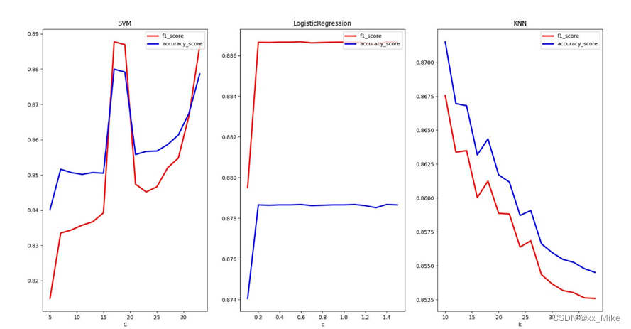
最后训练结果如下,每个方法都能达到85-90的准去率和f1得分,说明特征选取较为合适,其中最高得分和准确率为支持向量机方法,分别为0.887和0.879
代码整理
这里贴出详细实现代码:
1.文本预处理类textPreprossing.py:主要包含词频表生成,特征工程建立等
'''文本分类预处理,包含文本提取,'''
import numpy as np
import pandas as pd
import os
import re
import pickle

class config:
    def __init__(self,path,runBatch,saveName,stopWordsPath,posPath,negPath,posVocabfPath,negVocabfPath):
        self.path = path
        self.runBatch = runBatch
        self.stopWordsPath = stopWordsPath
        self.saveName = saveName
        self.posPath = posPath
        self.negPath = negPath
        self.posVocabfPath = posVocabfPath
        self.negVocabfPath = negVocabfPath

class textPre:

    def __init__(self,config):
        self.loadPath = config.path
        self.stopWords = []
        with open(config.stopWordsPath, encoding= "utf-8") as sf:
            for line in sf.readlines():
                self.stopWords.append(line.replace("\n",""))
        print("停用词{}个,{}个待读取文件".format(len(self.stopWords), len(os.listdir(self.loadPath))))
        # print(self.stopWords)
        # print(self.textNameList)

    '''生成语料表'''
    def create_vocab(self,config):
        vocab_dict = {}
        vocab_dict_num = 0
        loadPath = config.path
        runBatch = config.runBatch
        textNum = 0
        vocabList = ""
        count = 1
        sumCount = 1
        textNameList = os.listdir(loadPath)
        for textName in textNameList:
            loadPathCash = loadPath + "/pos" + "/" + textName
            if textNum != len(textNameList):
                if (textNum % runBatch != 0 or textNum == 0) :
                    with open(loadPathCash, encoding= "utf-8") as f:
                        vocabList = vocabList + " " +  f.read().lower()
                    textNum = textNum + 1
                    sumCount = sumCount + 1
                    continue
            # 去除符号,括号,以及停用词汇
            print("开始第{}批词语处理进入语料库,当前语料库共有{}个词汇".format(count, len(vocab_dict)))
            vocabList = re.sub("\<.*?\>",'',vocabList)
            vocabList = re.sub("\(.*?\)",'',vocabList)
            vocabList = re.sub("\[.*?\]",'',vocabList)
            vocabList = re.sub('[0-9’!"#$%&\'()*+,-./:;<=>?@,。?★、…【】《》?“”‘’![\\]^_`{|}~]+', '', vocabList)
            vocabList = vocabList.replace(","," ").replace("."," ").replace("'"," ").replace('"'," ").split()
            for vocab in vocabList:
                if vocab not in self.stopWords and vocab not in vocab_dict.keys():
                    vocab_dict[vocab] = vocab_dict_num + 1
                    vocab_dict_num = vocab_dict_num + 1
            vocabList = ""
            count = count + 1
            textNum = 0
        dict_save = open('vocab_dict.pkl','wb')
        pickle.dump(vocab_dict , dict_save)

    '''生成词频表'''
    def create_vocabf(self,config):
        vocabf_dict = {}
        vocabf_dict_num = 0
        loadPath = config.path
        runBatch = config.runBatch
        textNum = 0
        vocabList = ""
        count = 1
        sumCount = 1
        textNameList = os.listdir(loadPath)
        for textName in textNameList:
            loadPathCash = loadPath +  "/" + textName
            if textNum != len(textNameList):
                if (textNum % runBatch != 0 or textNum == 0):
                    with open(loadPathCash, encoding="utf-8") as f:
                        vocabList = vocabList + " " + f.read().lower()
                    textNum = textNum + 1
                    sumCount = sumCount + 1
                    continue
            # 去除符号,括号,以及停用词汇
            print("开始第{}批词语处理进入语料库,当前语料库共有{}个词汇".format(count, len(vocabf_dict)))
            vocabList = re.sub("\<.*?\>", '', vocabList)
            vocabList = re.sub("\(.*?\)", '', vocabList)
            vocabList = re.sub("\[.*?\]", '', vocabList)
            vocabList = re.sub('[0-9’!"#$%&\'()*+,-./:;<=>?@,。?★、…【】《》?“”‘’![\\]^_`{|}~]+','',vocabList)
            vocabList = vocabList.replace(",", " ").replace(".", " ").replace("'", " ").replace('"', " ").split()
            for vocab in vocabList:
                # 过滤停用词
                if vocab not in self.stopWords:
                    # 不在字典则添加,否则增加频数
                    if vocab not in vocabf_dict.keys():
                        vocabf_dict[vocab] = 1
                        vocabf_dict_num = vocabf_dict_num + 1
                    else:
                        vocabf_dict[vocab] = vocabf_dict[vocab] + 1

            vocabList = ""
            count = count + 1
            textNum = 0
        dict_save = open(config.saveName + '.pkl', 'wb')
        pickle.dump(vocabf_dict, dict_save)


    '''文本读取:生成np矩阵,特征选取:1 积极性词汇出现总数 2 消极性词汇出现总数 3 积极性词汇信息熵 4 消极性词汇信息熵'''
    def textBatchLoad(self,config , choose):
        featureInput = []
        if choose:
            textLoadPath = config.posPath
        else:
            textLoadPath = config.negPath
        textNameList = os.listdir(textLoadPath)
        f_read = open(config.posVocabfPath, 'rb')
        posDict = pickle.load(f_read)
        f_read = open(config.negVocabfPath, 'rb')
        negDict = pickle.load(f_read)
        f_read.close()
        count = 0
        for text in textNameList:
            if count % 50 == 0:
                print("开始处理第{}个文本".format(count))
            with open(textLoadPath + '/' + text, encoding= 'gbk' ,errors= 'ignore') as f:
                vocabList = f.read().lower()
                vocabList = re.sub("\<.*?\>", '', vocabList)
                vocabList = re.sub("\(.*?\)", '', vocabList)
                vocabList = re.sub("\[.*?\]", '', vocabList)
                vocabList = vocabList.replace(",", " ").replace(".", " ").replace("'", " ").replace('"', " ")
                vocabList = re.sub('[0-9’!"#$%&\'()*+,-./:;<=>?@,。?★、…【】《》?“”‘’![\\]^_`{|}~]+', '', vocabList).split()
            posCount = 0
            negCount = 0
            posCross = 0
            negCross = 0
            cashList = []
            featureInputCash = []
            for vocab in vocabList:
                if vocab not in cashList:
                    if vocab in posDict:
                        posCount = posCount + vocabList.count(vocab)
                        posCross = posCross + \
                                   (vocabList.count(vocab)/posDict[vocab])*np.log((vocabList.count(vocab)/posDict[vocab]))
                    if vocab in negDict:
                        negCount = negCount + vocabList.count(vocab)
                        negCross = negCross + \
                                   (vocabList.count(vocab) / negDict[vocab]) * np.log((vocabList.count(vocab) / negDict[vocab]))
                cashList.append(vocab)
            featureInputCash.append(posCount)
            featureInputCash.append(negCount)
            featureInputCash.append(posCross)
            featureInputCash.append(negCross)
            if choose == 1:
                featureInputCash.append(1)
            else:
                featureInputCash.append(0)
            featureInput.append(featureInputCash)
            count = count + 1
        return np.array(featureInput)


# path = "./dataset/txt_sentoken/neg"
# stopWordsPath = "./stopwords.txt"
# config = config(path = path,runBatch=50,saveName = "vocab_txtf_neg_dict",
#                 stopWordsPath = stopWordsPath, posPath="./dataset/train/neg", negPath="./dataset/train/neg",
#                 posVocabfPath= "./vocabf_pos_dict.pkl", negVocabfPath= "./vocabf_neg_dict.pkl")
# textPres = textPre(config)
# textPres.create_vocabf(config)
2.模型训练mashineLearningForText.py:进行模型训练
import sklearn
import sklearn.svm as svm
import numpy as np
import math
from data import textPreprossing as tPre
from sklearn.metrics import f1_score
from sklearn.metrics import accuracy_score
from sklearn.preprocessing import MinMaxScaler
from sklearn.model_selection import KFold
import matplotlib.pyplot as plt
from sklearn.linear_model import LogisticRegression
from sklearn.neighbors import KNeighborsClassifier


# path = "../data/dataset/train/unsup"
# stopWordsPath = "../data/stopwords.txt"
# configTrain = tPre.config(path = path,runBatch=50,saveName = "vocabf_unsup_dict",
#                 stopWordsPath = stopWordsPath, posPath="../data/dataset/train/pos", negPath="../data/dataset/train/neg",
#                 posVocabfPath= "../data/vocabf_pos_dict.pkl", negVocabfPath= "../data/vocabf_neg_dict.pkl")
# configTest = tPre.config(path = path,runBatch=50,saveName = "vocabf_unsup_dict",
#                 stopWordsPath = stopWordsPath, posPath="../data/dataset/test/pos", negPath="../data/dataset/test/neg",
#                 posVocabfPath= "../data/vocabf_pos_dict.pkl", negVocabfPath= "../data/vocabf_neg_dict.pkl")
# textPres = tPre.textPre(configTrain)
# testPres = tPre.textPre(configTest)
# # input1 = textPres.textBatchLoad(configTrain,1)
# # input2 = textPres.textBatchLoad(configTrain,2)
# train = sklearn.utils.shuffle(np.vstack((textPres.textBatchLoad(configTrain,1) , textPres.textBatchLoad(configTrain,0))))
# test = sklearn.utils.shuffle(np.vstack((testPres.textBatchLoad(configTrain,1) , testPres.textBatchLoad(configTrain,0))))
# # 保存数据,避免重复处理,提高效率
# np.save("../data/lmdb_train",train)
# np.save("../data/lmdb_test",test)

# 加载数据
train = np.load("../data/lmdb_train.npy")
test = np.load("../data/lmdb_test.npy")
# data = np.load("../data/txt_data.npy")

# 十则交叉验证
kf = KFold(n_splits = 10 )
data = np.vstack((train,test))
scaler = MinMaxScaler()

# 归一化
data[:,0:4] = scaler.fit_transform(data[:,0:4])

print("归一化样例:{}".format(data[0:10]))

f1_score_diedai = []
accuracy_score_diedai = []
f1_score_logDiedai = []
accuracy_score_logDiedai = []
f1_score_knnDiedai = []
accuracy_score_knnDiedai = []


for c in range(5,20):
    f1_score_list = []
    accuracy_score_list = []
    f1_score_logList = []
    accuracy_score_logList = []
    f1_score_knnList = []
    accuracy_score_knnList = []

    count = 1
    for train_index,test_index in kf.split(data):
        print("开始交叉验证第{}次,C = {}".format(count,c))
        train = data[train_index]
        test = data[test_index]
        # 支持向量机 SVM
        svm_model = svm.SVC(C= 2 * (c-5)+5, kernel= 'linear')
        # 逻辑回归
        log_model = LogisticRegression(penalty='l1', C=c/10-0.4, solver='liblinear')
        #多项式贝叶斯
        knn_model = KNeighborsClassifier(n_neighbors= 10 + (c-5)*2)

        svm_model.fit(train[:,0:4],train[:,4])
        log_model.fit(train[:,0:4],train[:,4])
        knn_model.fit(train[:,0:4],train[:,4])
        # 预测
        pre_y = np.array(svm_model.predict(test[:,0:4]))
        pre_y_log = np.array(log_model.predict(test[:,0:4]))
        pre_y_bayes = np.array(knn_model.predict(test[:,0:4]))
        # svm
        f1_score_test = f1_score(y_true = test[:,4],y_pred = pre_y)
        accuracy_score_test = accuracy_score(y_true = test[:,4],y_pred = pre_y)

        # 逻辑回归
        f1_score_logTest = f1_score(y_true=test[:, 4], y_pred=pre_y_log)
        accuracy_score_logTest = accuracy_score(y_true=test[:, 4], y_pred=pre_y_log)

        # KNN
        f1_score_knnTest = f1_score(y_true=test[:,4] , y_pred=pre_y_bayes)
        accuracy_score_knnTest = accuracy_score(y_true=test[:,4],y_pred=pre_y_bayes)

        f1_score_list.append(f1_score_test)
        accuracy_score_list.append(accuracy_score_test)
        f1_score_logList.append(f1_score_logTest)
        accuracy_score_logList.append(accuracy_score_logTest)
        f1_score_knnList.append(f1_score_knnTest)
        accuracy_score_knnList.append(accuracy_score_knnTest)
        print("SVM:f1_score:{},accuracy_score:{}\n"
              "逻辑回归:f1_score:{},accuracy_score:{}\n"
              "knn:f1_score:{},accuracy_score:{}"
              .format(f1_score_test, accuracy_score_test,
                      f1_score_logTest,accuracy_score_logTest,
                    f1_score_knnTest,accuracy_score_knnTest))
        count = count + 1

    f1_score_diedai.append(np.mean(np.array(f1_score_list)))
    accuracy_score_diedai.append(np.mean(np.array(accuracy_score_list)))
    f1_score_logDiedai.append(np.mean(np.array(f1_score_logList)))
    accuracy_score_logDiedai.append(np.mean(np.array(accuracy_score_logList)))
    f1_score_knnDiedai.append(np.mean(np.array(f1_score_knnList)))
    accuracy_score_knnDiedai.append(np.mean(np.array(accuracy_score_knnList)))

    print("SVM(C={}):f1_score_avr:{},accuracy_score_avr:{}\n"
          "逻辑回归(c={}):f1_score_avr:{},accuracy_score_avr:{}\n"
          "knn(k={}):f1_score_avr:{},accuracy_score_avr:{}".
          format(c,np.mean(np.array(f1_score_list)),np.mean(np.array(accuracy_score_list)),
          (c-0.5)/10,np.mean(np.array(f1_score_logList)),np.mean(np.array(accuracy_score_logList)),
          10+(c-5)*2,np.mean(np.array(f1_score_knnList)),np.mean(np.array(accuracy_score_knnList))))
    #
print("SVM:f1_score_diedai:{},accuracy_score_diedai:{}\n"
      "逻辑回归:f1_score_diedai:{},accuracy_score_diedai:{}\n"
      "knn:f1_score_diedai:{},accuracy_score_diedai:{}".
      format(f1_score_diedai,accuracy_score_diedai,
             f1_score_logDiedai,accuracy_score_logDiedai,
             f1_score_knnDiedai,accuracy_score_knnDiedai))


print("训练结束,开始绘图...")
# 绘图
x = [5,7,9,11,13,15,17,19,21,23,25,27,29,31,33]
x_log = [0.1,0.2,0.3,0.4,0.5,0.6,0.7,0.8,0.9,1,1.1,1.2,1.3,1.4,1.5]
x_bayes = [10,12,14,16,18,20,22,24,26,28,30,32,34,36,38]

# SVM
plt.subplot(1,3,1)
plt.plot(x,f1_score_diedai,color = 'red',label = "f1_score",linewidth = 2.5)
plt.plot(x,accuracy_score_diedai, color = 'blue',label = "accuracy_score",linewidth = 2.5)
plt.xlabel("C")
plt.legend(loc = 'upper right')
plt.title("SVM")

# 逻辑回归
plt.subplot(1,3,2)
plt.plot(x_log,f1_score_logDiedai,color = 'red',label = "f1_score",linewidth = 2.5)
plt.plot(x_log,accuracy_score_logDiedai, color = 'blue',label = "accuracy_score",linewidth = 2.5)
plt.xlabel("c")
plt.legend(loc = 'upper right')
plt.title("LogisticRegression")

# 朴素贝叶斯
plt.subplot(1,3,3)
plt.plot(x_bayes,f1_score_knnDiedai,color = 'red',label = "f1_score",linewidth = 2.5)
plt.plot(x_bayes,accuracy_score_knnDiedai, color = 'blue',label = "accuracy_score",linewidth = 2.5)
plt.legend(loc = 'upper right')
plt.xlabel("k")
plt.title("KNN")

plt.show()
附录
- 停用词整理:
'd
'll
'm
're
's
't
've
ZT
ZZ
a
a's
able
about
above
abst
accordance
according
accordingly
across
act
actually
added
adj
adopted
affected
affecting
affects
after
afterwards
again
against
ah
ain't
all
allow
allows
almost
alone
along
already
also
although
always
am
among
amongst
an
and
announce
another
any
anybody
anyhow
anymore
anyone
anything
anyway
anyways
anywhere
apart
apparently
appear
appreciate
appropriate
approximately
are
area
areas
aren
aren't
arent
arise
around
as
aside
ask
asked
asking
asks
associated
at
auth
available
away
awfully
b
back
backed
backing
backs
be
became
because
become
becomes
becoming
been
before
beforehand
began
begin
beginning
beginnings
begins
behind
being
beings
believe
below
beside
besides
best
better
between
beyond
big
biol
both
brief
briefly
but
by
c
c'mon
c's
ca
came
can
can't
cannot
cant
case
cases
cause
causes
certain
certainly
changes
clear
clearly
co
com
come
comes
concerning
consequently
consider
considering
contain
containing
contains
corresponding
could
couldn't
couldnt
course
currently
d
date
definitely
describe
described
despite
did
didn't
differ
different
differently
discuss
do
does
doesn't
doing
don't
done
down
downed
downing
downs
downwards
due
during
e
each
early
ed
edu
effect
eg
eight
eighty
either
else
elsewhere
end
ended
ending
ends
enough
entirely
especially
et
et-al
etc
even
evenly
ever
every
everybody
everyone
everything
everywhere
ex
exactly
example
except
f
face
faces
fact
facts
far
felt
few
ff
fifth
find
finds
first
five
fix
followed
following
follows
for
former
formerly
forth
found
four
from
full
fully
further
furthered
furthering
furthermore
furthers
g
gave
general
generally
get
gets
getting
give
given
gives
giving
go
goes
going
gone
good
goods
got
gotten
great
greater
greatest
greetings
group
grouped
grouping
groups
h
had
hadn't
happens
hardly
has
hasn't
have
haven't
having
he
he's
hed
hello
help
hence
her
here
here's
hereafter
hereby
herein
heres
hereupon
hers
herself
hes
hi
hid
high
higher
highest
him
himself
his
hither
home
hopefully
how
howbeit
however
hundred
i
i'd
i'll
i'm
i've
id
ie
if
ignored
im
immediate
immediately
importance
important
in
inasmuch
inc
include
indeed
index
indicate
indicated
indicates
information
inner
insofar
instead
interest
interested
interesting
interests
into
invention
inward
is
isn't
it
it'd
it'll
it's
itd
its
itself
j
just
k
keep
keeps
kept
keys
kg
kind
km
knew
know
known
knows
l
large
largely
last
lately
later
latest
latter
latterly
least
less
lest
let
let's
lets
like
liked
likely
line
little
long
longer
longest
look
looking
looks
ltd
m
made
mainly
make
makes
making
man
many
may
maybe
me
mean
means
meantime
meanwhile
member
members
men
merely
mg
might
million
miss
ml
more
moreover
most
mostly
mr
mrs
much
mug
must
my
myself
n
n't
na
name
namely
nay
nd
near
nearly
necessarily
necessary
need
needed
needing
needs
neither
never
nevertheless
new
newer
newest
next
nine
ninety
no
nobody
non
none
nonetheless
noone
nor
normally
nos
not
noted
nothing
novel
now
nowhere
number
numbers
o
obtain
obtained
obviously
of
off
often
oh
ok
okay
old
older
oldest
omitted
on
once
one
ones
only
onto
open
opened
opening
opens
or
ord
order
ordered
ordering
orders
other
others
otherwise
ought
our
ours
ourselves
out
outside
over
overall
owing
own
p
page
pages
part
parted
particular
particularly
parting
parts
past
per
perhaps
place
placed
places
please
plus
point
pointed
pointing
points
poorly
possible
possibly
potentially
pp
predominantly
present
presented
presenting
presents
presumably
previously
primarily
probably
problem
problems
promptly
proud
provides
put
puts
q
que
quickly
quite
qv
r
ran
rather
rd
re
readily
really
reasonably
recent
recently
ref
refs
regarding
regardless
regards
related
relatively
research
respectively
resulted
resulting
results
right
room
rooms
run
s
said
same
saw
say
saying
says
sec
second
secondly
seconds
section
see
seeing
seem
seemed
seeming
seems
seen
sees
self
selves
sensible
sent
serious
seriously
seven
several
shall
she
she'll
shed
shes
should
shouldn't
show
showed
showing
shown
showns
shows
side
sides
significant
significantly
similar
similarly
since
six
slightly
small
smaller
smallest
so
some
somebody
somehow
someone
somethan
something
sometime
sometimes
somewhat
somewhere
soon
sorry
specifically
specified
specify
specifying
state
states
still
stop
strongly
sub
substantially
successfully
such
sufficiently
suggest
sup
sure
t
t's
take
taken
taking
tell
tends
th
than
thank
thanks
thanx
that
that'll
that's
that've
thats
the
their
theirs
them
themselves
then
thence
there
there'll
there's
there've
thereafter
thereby
thered
therefore
therein
thereof
therere
theres
thereto
thereupon
these
they
they'd
they'll
they're
they've
theyd
theyre
thing
things
think
thinks
third
this
thorough
thoroughly
those
thou
though
thoughh
thought
thoughts
thousand
three
throug
through
throughout
thru
thus
til
tip
to
today
together
too
took
toward
towards
tried
tries
truly
try
trying
ts
turn
turned
turning
turns
twice
two
u
un
under
unfortunately
unless
unlike
unlikely
until
unto
up
upon
ups
us
use
used
useful
usefully
usefulness
uses
using
usually
uucp
v
value
various
very
via
viz
vol
vols
vs
w
want
wanted
wanting
wants
was
wasn't
way
ways
we
we'd
we'll
we're
we've
wed
welcome
well
wells
went
were
weren't
what
what'll
what's
whatever
whats
when
whence
whenever
where
where's
whereafter
whereas
whereby
wherein
wheres
whereupon
wherever
whether
which
while
whim
whither
who
who'll
who's
whod
whoever
whole
whom
whomever
whos
whose
why
widely
will
willing
wish
with
within
without
won't
wonder
words
work
worked
working
works
world
would
wouldn't
www
x
y
year
years
yes
yet
you
you'd
you'll
you're
you've
youd
young
younger
youngest
your
youre
yours
yourself
yourselves
z
zero
zt
zz


 1349
1349

 被折叠的 条评论
为什么被折叠?
被折叠的 条评论
为什么被折叠?
 到【灌水乐园】发言


