GCN:基于切比雪夫多项式(chebyshev ploynomials)为核的图卷积推导与pytorch实现

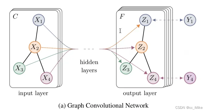
GCN图卷积神经网络

顾名思义，图卷积神经网络，是对图信息进行卷积，从而获取相邻节点的信息和特征，本文将介绍和推导目前较为流行的以chebyshev ploynomials 契比雪夫多项式为核的图卷积公式，同时通过pytorch代码实现。

图卷积的定义

通过表示图信息的矩阵及上一层特征输入，输出该层对图信息的特征，表示如下：
$H_l=f(H_{l-1},A)$
A代表邻接矩阵，或关于图表示的矩阵。
常用数学传播表示方式如下：
$$H_l=\sigma ({\tilde{D}}^{-\frac{1}{2}}\tilde{A}{\tilde{D}}^{-\frac{1}{2}}{H}_{l-1}{W}_{l-1})$$

其中$\tilde{D}$代表$\tilde{A}$的度矩阵

$\tilde{A}$代表邻接矩阵$A$与单位矩阵$I$的和:$\tilde{A}=A+I$

$H$代表卷积后的特征，初始输入$H=X$

$\sigma$为激活函数

推导

1. 图的表示方式：

   1）邻接矩阵$A$，表示节点与节点之间是否存在连接，若存在则为1，不存在为0，对角线均为0

   2）度矩阵$D$ ，只有对角线有值，表示该节点所连接边的个数

   ​3） Laplacian 拉普拉斯矩阵：$L=D-A$ 1)对称 2）非负特征值 3）正交

   ​ 归一化Laplacian: $L^{sym}=D^{-\frac{1}{2}}L{D}^{-\frac{1}{2}}=I-D^{-\frac{1}{2}}A{D}^{-\frac{1}{2}}$

2. 卷积公式:其中$F(X)$表示傅里叶变换

   $f\ast g=F^{-1}(F(f)\ast F(g))$

3. 根据拉普拉斯矩阵正交特性，存在$U,U^T$使得$L=U\Lambda U^T$ 其中$\Lambda$表示特征向量

   则Graph Fourier可对应表示如下：

   $GF(x)=U^{T}x$

   根据卷积公式，对应图卷积公式如下：

   $g\ast x=U(U^{T}g{U}^{T}x)$

   每一次卷积操作作用域都希望在中心节点附近的区域，则我们可以将$g$看作关于拉普拉斯矩阵$L$的函数$g(L)$，那么，每卷积一次则相当于传递一次相邻节点信息

   而由$L$特征值特性：$U^{T}L=\Lambda U^T$ 可知，$U^{T}g(L)$ 可看作是关于拉普拉斯矩阵$L$的特征函数$g_{\theta }(\Lambda )$

   则图卷积表达式可写作：

   $g\ast x=U(U^{T}g{U}^{T}x)=U{g}_{\theta }{U}^{T}x$

4. 运算简化

   由于计算$g_{\theta }$需要计算拉普拉斯矩阵特征值，计算复杂，因而提出利用切比雪夫Chebyshev polynomials多项式来进行近似计算，这里并不影响特征值的计算属性，只是通过切比雪夫多项式作为核能够将特征值矩阵计算化简为L，从而跳过特征值计算的步骤，表示如下。

   $g_{\theta }={\sum }_{k=0}^K{\theta }_k{T}_k(\tilde{\Lambda })$

   其中$\tilde{\Lambda }=2\ast \frac{\Lambda }{{\Lambda }_{max}}-1$,只是因为Chebyshev polynomials要求$x$处于$[-1,1]$

   $T_k(x)=2x{T}_{k-1}(x)-T_{k-2}(x)$,$T_0=0$,$T_1=1$

   那么将上式代入卷积表达式可以得到：

   $$\begin{gathered} g\ast x=U\sum _{k=0}^K{\theta }_k{T}_k(\tilde{\Lambda })U^{T}x \\ =\sum _{k=0}^K{\theta }_K{T}_k(\tilde{L})x \end{gathered}$$

pytorch代码实现

包需求：

import numpy as np
import torch
import torch.nn as nn

1.Laplacian 以及scaled_Laplacian:

'''D matrix 根据邻接矩阵获取度矩阵'''
def get_d_matrix(adj_matrix):
    d_matrix = np.zeros((adj_matrix.shape[0], adj_matrix.shape[1]))
    for i in range(adj_matrix.shape[0]):
        d_matrix[i, i] = np.sum(adj_matrix[i, :])
    return d_matrix

'''Laplace matrix'''
def get_laplace_matrix(adj, d):
    d_turn = np.zeros((adj.shape[0], adj.shape[0]))
    for i in range(adj.shape[0]):
        d_turn[i, i] = np.power(d[i, i], -0.5)
    res = np.eye(adj.shape[0]) - d_turn @ adj @ d_turn
    return res


'''
get the  rou of matrix 获取矩阵谱半径，即最大绝对值特征值
'''
def getRou(x):
    lambdas, features = np.linalg.eig(x)
    return np.max(np.abs(lambdas))

'''
get scaled laplacian for chebyshev ploynomials
'''
def scaled_laplacian(L):
    res = (2*L)/getRou(L)-np.identity(L.shape[0])
    return res

2. 契比雪夫多项式的实现

'''
get chebyshev ploynomials 
'''
def chebyshev_ploynomials(scaled_laplacian, K):
    '''
    :param scaled_laplacian: [-1，1]的拉普拉斯矩阵
    :param K: 多项式项数
    :return: list
    '''
    res = [np.identity(scaled_laplacian.shape[0]), scaled_laplacian]
    if K>=2:
        for i in range(2, K+1):
            res.append(2*scaled_laplacian*res[i-1]-res[i-2])
    return res

3. pytorch 实现图卷积

'''
take chebyshev ploynomials as kernal for graph conv
'''
class Cheb_conv(nn.Module):
    def __init__(self, chebyshev_ploynomials, K, in_channel, out_channel):
        super(Cheb_conv, self).__init__()
        self.K = K
        self.chebyshev_ploynomials = chebyshev_ploynomials
        self.device = chebyshev_ploynomials[0].device
        self.thetaList = nn.ParameterList([nn.Parameter(torch.FloatTensor(in_channel, out_channel).to(self.device)) for _ in range(K)])
        self.relu = nn.ReLU()

    def forward(self, x):
        '''

        :param x: (batch, nodes_num, features(in_channel), seq_len)
        :return:
        '''
        batch_size, nodes_num, in_channel, seq_len = x.shape
        #(batch, seq_len, nodes_num, in_channel)
        x = x.permute(0,3,1,2)
        output = torch.zeros(batch_size, nodes_num, self.out_channels, seq_len).to(self.DEVICE)
        for i in range(self.K):
            cheb = self.chebyshev_ploynomials[i]
            #(batch, seq_len, nodes_num, in_channel)
            cash = cheb.matmul(x)
            # (batch, seq_len, nodes_num, out_channel)
            cash = self.cash.matmul(self.thetaList[i])
            #(batch, nodes_num, out_channel, seq_len)
            cash = cash.permute(0,2,3,1)
            output += cash

        return self.relu(output)