3.分类问题---手写数字识别初体验

分类问题引入

MNIST

每张图片大小是28*28
矩阵[28，28]->[784]->[1,784],二维变成一维的。

loss

H3：[1,1],第一个1是图片数量，第二个1表示0-9的数字
Y：[0/1/,/9]，采用one_hot，如果它的标签是3->[0,0,0,3,0,0,0,0,0]
假如图片上的数字是5，则H3可能是[0.1,0.0.01,0.01,0.03,0.01,0.8,0.01,0.01,0.01,0.01],实际上的Y应该是[0,0,0,0,0,1,0,0,0,0]。

H3	0.1	0.01	0.01	0.03	0.01	0.8	0.01	0.01	0.01	0.01
Y	0	0	0	0	0	1	0	0	0	0

loss采用欧氏距离公式计算

梯度下降

H1=relu(W1x+b1)
H2=relu(W2H1+b2)
H3=W3*H2+b3
pred=H3
out = Σ(pred-Y)**2

结果

argmax(pred)：最大值返回所在索引

手写数字初体验

1.数据加载（Load data）

batch_size = 512
train_loader = torch.utils.data.DataLoader(
    torchvision.datasets.MNIST('mnist_data', train=True, download=True,
                               transform=torchvision.transforms.Compose([
                                   torchvision.transforms.ToTensor(),
                                   torchvision.transforms.Normalize(
                                       (0.1307,), (0.3081,))
                               ])),
    batch_size=batch_size, shuffle=True)
# 把numpy格式转换成tensor
# 正则化，在0附近，可提升性能
test_loader = torch.utils.data.DataLoader(
    torchvision.datasets.MNIST('mnist_data/', train=False, download=True,
                               transform=torchvision.transforms.Compose([
                                   torchvision.transforms.ToTensor(),
                                   torchvision.transforms.Normalize(
                                       (0.1307,), (0.3081,))
                               ])),
    batch_size=batch_size, shuffle=False)

x, y = next(iter(train_loader))
print(x.shape, y.shape, x.min(), x.max())
plot_image(x, y, 'image sample')

2.创建模型（Build Model）

class Net(nn.Module):

    def __init__(self):
        super(Net,self).__init__()

        #wx+b
        self.fc1 = nn.Linear(28*28,256)  #，28*28是x的维度，256一般根据经验随机决定，大维变成小维
        self.fc2 = nn.Linear(256,64)     #第二层的输入与上一层的输出相同
        self.fc3 = nn.Linear(64,10)      #10分类，此处不是根据经验

    #计算过程
    def forward(self,x):
        # x: [b,1,28,28]
        # h1 =relu(xw1+b1)
        x = F.relu(self.fc1(x))
        # h2 = relu(h1w2+b2)
        x = F.relu(self.fc2(x))
        # h3 = h2w3+b3,最后一层看情况添加激活函数
        x = self.fc3(x)

        return x

3.训练（Train）

#train
#net.parameters()返回[w1,b1,w2,b2,w3,b3],这就是我们要优化的; lr是学习步长 ;momentum帮助更好的优化
net = Net()
optimizer = optim.SGD(net.parameters(),lr=0.01,momentum=0.9)

#把loss保存起来
train_loss = []

for epoch in range(3):
    for batch_idx, (x,y) in enumerate(train_loader):

        # x: [b,1,28,28]  y : [512]
        # [b,1,28,28]打平成[b,feature],size(0)是batch
        x = x.view(x.size(0),28*28)
        #成[b,10]
        out = net(x)
        # [b,10],真实的y
        y_onehot= one_hot(y)
        # loss=mse(out,y_onehot),求其均方差
        loss = F.mse_loss(out,y_onehot)

        #清零梯度
        optimizer.zero_grad()
        #计算梯度
        loss.backward()
        # 更新梯度：w‘ = w-lr*grad
        optimizer.step()

        #进行梯度下降的可视化，把数据记录下来
        train_loss.append(loss.item())

        if batch_idx % 10 == 0:
            print(epoch,batch_idx,loss.item())

plot_curve(train_loss)
#we can get optimal [w1,b1,w2,b2,w3,b3]

4.测试（Test）

total_correct = 0
for x,y in test_loader:
    x = x.view(x.size(0),28*28)
    #out : [b,10]
    out = net(x)
    #out -> pred:[b]
    pred =out.argmax(dim=1)
    #当前预测对的数量的总和转成float,此时还是tensor类型，再转换成数值类型
    correct = pred.eq(y).sum().float().item()
    total_correct += correct

total_num = len(test_loader.dataset)
acc = total_correct / total_num
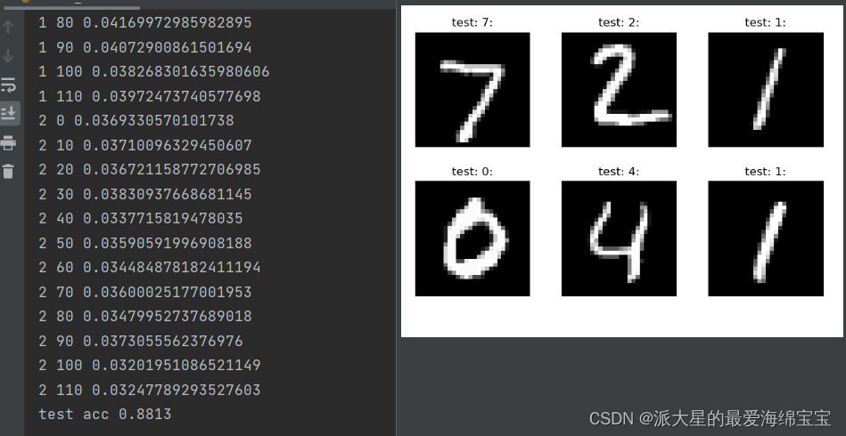
print('test acc', acc)

x,y = next(iter(test_loader))
out = net(x.view(x.size(0),28*28))
pred =out.argmax(dim=1)
plot_image(x,pred,'test')