逻辑回归

一、导入使用模块

import pandas as pd
import numpy as np
import matplotlib.pyplot as plt
import seaborn as sns#画图工具，在matplot上进行API精装
plt.style.use('fivethirtyeight') #样式美化
import matplotlib.pyplot as plt
# import tensorflow as tf
from sklearn.metrics import classification_report#这个包是评价报告

二、导入数据

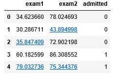
data = pd.read_csv('F:\\MachineLearning\data\ex2data1.txt', names=['exam1', 'exam2', 'admitted'])
data.head()#看前五行

read_csv中的参数names以列表形式给每一列命名。

如图所示为数据形式：

下面为数据展示：

sns.set(context='notebook',style='darkgrid')                  #context:设置绘图元素大小（坐标轴标记大小），style:主题风格
sns.set_palette(palette=sns.color_palette("RdBu", 2)) #设置分类色板
sns.lmplot('exam1','exam2',hue='admitted',data=data,height=6,fit_reg=False,scatter_kws={"s": 50})#exam1,exam2:分别在制定的行列上分类
#hua:用于分类的属性，size：设置图的大小，fig_reg:是否显示分类直线，scatter_kws:点的样式大小
plt.show()

得到点图为：

color_palette() 中的第一个参数为颜色风格，第二个参数为色块数。fit_reg表示是否要画出回归曲线。

三、数据处理

def get_X(df):#读取特征

    ones = pd.DataFrame({'ones': np.ones(len(df))})#ones所对应的列长度为m全为1
    data = pd.concat([ones, df], axis=1)  # 合并数据，根据列合并
    return data.iloc[:, :-1].as_matrix()  # 这个操作返回 ndarray,不是矩阵


def get_y(df):#读取标签
    return np.array(df.iloc[:, -1])        #df.iloc[:, -1]是指df的最后一列


def normalize_feature(df):

    return df.apply(lambda column: (column - column.mean()) / column.std())#特征缩放

由于要处理逻辑回归中常数项所对应的参数，所以要在X中的第一列添加全为1的列。concact将ones与df合并，axis=1表示按照行的方向合并。最会X除去倒数第一列。y则要取最后一列。normalize_feature为对数据进行归一化，防止在梯度下降过程中迭代过慢。
检查处理后数据的行数和列数：

X = get_X(data)
print(X.shape)

y = get_y(data)
print(y.shape)

得到：

(100, 3)
(100,)

四、sigmoid 函数
sigmoid函数形如：

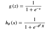
所以可以编写sigmoid函数的代码：

def sigmoid(z):
    return 1/(1+np.exp(-z))

然后展示sigmoid函数的曲线图：

fig, ax = plt.subplots(figsize=(8, 6))
ax.plot(np.arange(-10, 10, step=0.01),
        sigmoid(np.arange(-10, 10, step=0.01)))
ax.set_ylim((-0.1,1.1))
ax.set_xlabel('z', fontsize=18)
ax.set_ylabel('g(z)', fontsize=18)
ax.set_title('sigmoid function', fontsize=18)
plt.show()

得到图：

五、代价函数
逻辑回归的代价函数为：

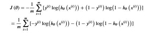
所以代价函数的代码如下：

def cost(theta, X, y):
    m=X.shape[0]
    sigVector=sigmoid(X@theta)
    totalCost=-(y@np.log(sigVector)+(1-y)@np.log(1-sigVector))
    return totalCost/m

下面检验其正确性：在这里插入代码片

theta = theta=np.zeros(3)
print(cost(theta, X, y))

得到代价函数的值为0.6931471805599452，发现正确。

六、计算梯度
梯度形式为：

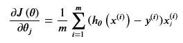
向量形式为：

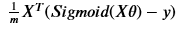
所以可以计算梯度：

def gradient(theta, X, y):
    m=X.shape[0]
    deltaVector=sigmoid(X@theta)-y
    grad=X.T@deltaVector/m
    return grad

七、拟合参数
这里我们不必编写梯度下降算法以得到最优值，只需调用scipy.optimize就可拟合最优值。代码如下：

import scipy.optimize as opt#拟合参数

res = opt.minimize(fun=cost, x0=theta, args=(X, y), method='Newton-CG', jac=gradient)#fun:需要最小化的函数。x0：最初的猜想，
#ndarray, shape (n,)。arg:需要传递给目标函数与及其倒数的参数，fun, jac and hess functions。method:所使用的方法。jac：梯度向量计算方法。

print(res)#res为一个字典，拥有以下属性。x : ndarra，问题的优化求解。success : bool，是否成功。status : int，优化器终止状态。
#message : str，终止状态的说明。fun, jac, hess: ndarray，目标函数的值。hess_inv : object，目标函数Hessian矩阵的逆。
#nfev, njev, nhev : int，目标函数及其雅可比矩阵和黑森矩阵的计算次数。nit : int，优化器执行的迭代次数。maxcv : float，最大约束冲突。

得到最终拟合状态：

fun: 0.2034977015894895
     jac: array([-4.33738420e-07, -2.47262193e-05, -2.84907400e-05])
 message: 'Optimization terminated successfully.'
    nfev: 72
    nhev: 0
     nit: 29
    njev: 256
  status: 0
 success: True
       x: array([-25.16135181,   0.20623186,   0.20147175])

于是最优化theta值为：

 array([-25.16135181,   0.20623186,   0.20147175])

八、用训练集预测和验证
用我们拟合得到参数带入逻辑回归，预测样本集中样本的类。首先编写prdict函数的到预测结果。

def predict(x, theta):
    fx=sigmoid(X@theta)
    pred_list=[]
    for a in fx:
        if a>=0.5:
            pred_list.append(1)
        else:
            pred_list.append(0)
    y_pred=np.array(pred_list)
    return y_pred

进行判断：

final_theta = res.x
y_pred=predict(X, final_theta)
print(type(y_pred))
print(classification_report(y, y_pred))

得到预测结果：

<class 'numpy.ndarray'>
              precision    recall  f1-score   support

           0       0.87      0.85      0.86        40
           1       0.90      0.92      0.91        60

   micro avg       0.89      0.89      0.89       100
   macro avg       0.89      0.88      0.88       100
weighted avg       0.89      0.89      0.89       100

得到判断0的精度为0.87，1的精度为0.9。

九、寻找决策边界
我们把我们拟合的参数作为决策边界的参数，查看拟合参数的拟合情况。

print(res.x)

[-25.16135181   0.20623186   0.20147175]

得到前面的拟合参数。

coef = -(res.x / res.x[2])  # find the equation
print(coef)

x = np.arange(130, step=0.1)
y = coef[0] + coef[1]*x

这一步主要是得到exam2属性关于exam1属性的函数。然后就可以通过曲线图得到拟合情况：

sns.set(context="notebook", style="ticks", font_scale=1.5)

sns.lmplot('exam1', 'exam2', hue='admitted', data=data, 
           size=6, 
           fit_reg=False, 
           scatter_kws={"s": 25}
          )

plt.plot(x, y, 'grey')
plt.xlim(0, 130)
plt.ylim(0, 130)
plt.title('Decision Boundary')
plt.show()