


 本文详细介绍了使用Simulink实现AM信号的调制与解调过程,包括语音信号的处理、数据速率转换及CIC滤波器的应用。同时,探讨了通过自定义S-function实现AM信号的正交解调,以及采用CORDIC算法进行角度检测和频差计算的方法。
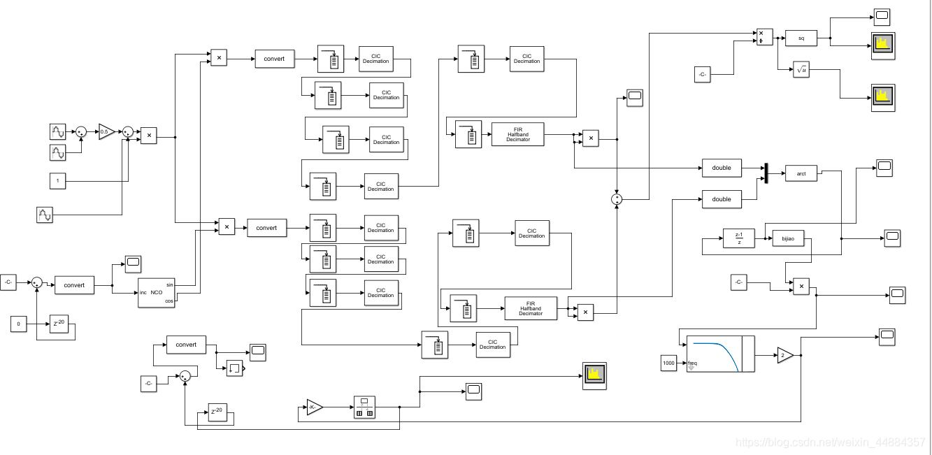
做出来的部分如上。由于是第一次用simulink,这里除了am信号通信部分,对simulink的使用理解也做一下简单记录。
1.调制发送
首先,信号发送部分,题目是语音信号,本来想自己录制一段语音进行发送接收,但是matlab读进来的音频信号采样频率是44100Hz,题目要求40M,差好多,数据采样速率转换,现在只知道找一个最小公倍数,先插值再抽取,用滤波器什么的不想去想了。所以最后就只用两个单频信号来表示语音信号,一个2k,一个3.4k.
am调制,防止过调制,将语音信号乘以0.5后再加上一个值为1的直流。然后乘以70M的载波。


这里频率是w,不要忘记乘以2*pi哦。
2.接收中的数据速率转换
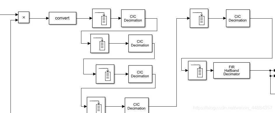
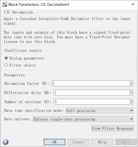
40M采样速率最后要求转换到8k,降低的倍数为5000=5x5x5x5x2x2x2.这里用cic和半带滤波器,半带滤波器,抽取倍数只能是2,所以前面cic的倍数分别是5,5,5,5,4.
看下图cic滤波器数据要求只能是fixed的,所以要有以后个convert数据类型转换。
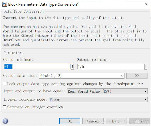
fixdt(1,12),1代表有符号数,12代表12为。
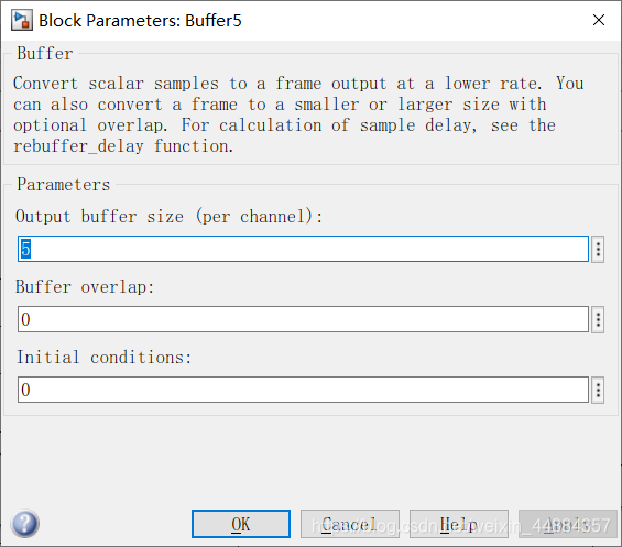
cic、半带滤波器前还需要一个buffer
3.解调
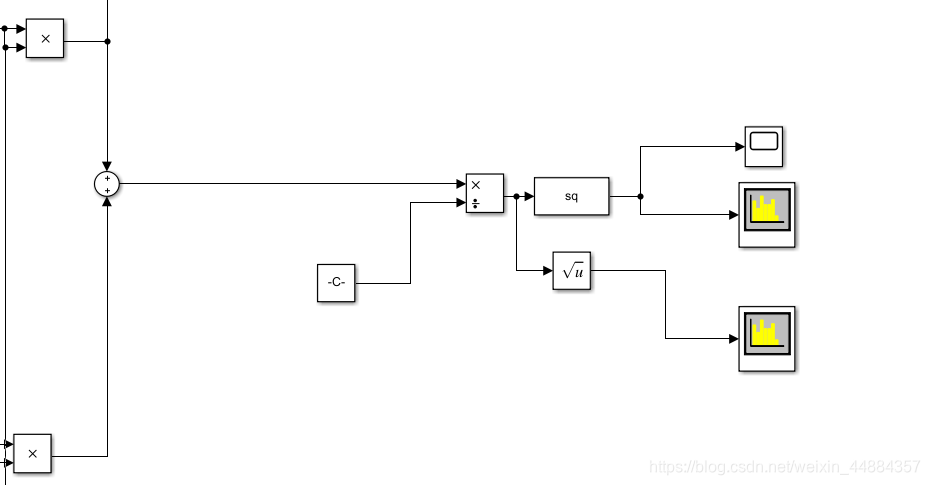
具体解调原理可以看AM信号的数字正交解调
就I ^2 + Q^2然后开根号。开根号是用的simulink的s-function,然后用的cordic算法自己写的。
在matlab命令行中编辑edit sfuntmpl就可以找到这个模板。需要更改的地方也不多。详细看
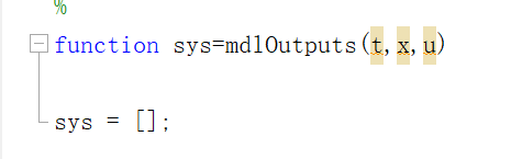
其中函数输入输出,t是采样时间,x是状态变量(这里没用到,就不用更改),u是输入,flag是仿真过程中的一个标志位,标识程序是在初始化状态还是运行状态。sys是函数输出。
模板中第一个更改的地方是:
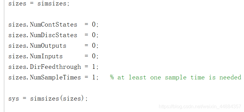
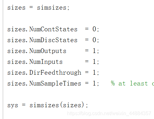
首先输入输出变量个数,开根号运算输入输出都是一个。
第二个更改采样时间
采样时间点的确定:下一个采样时间=(n*采样间隔)+ 偏移量,n表示当前的仿真步,从0开始。
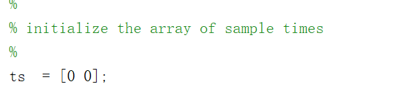
对于连续采样时间,ts可以设置为[0 0],其中偏移量为0;
对于离散采样时间,ts假设为[0.25 0.1],表示在S-函数仿真开始后0.1s开始每隔0.25s运行一次,当然每个采样时刻都会调用mdlOutPuts和mdlUpdate函数;
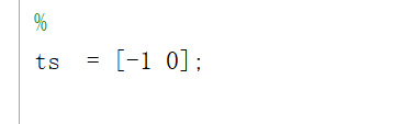
对于变采样时间,即离散采样时间的两次采样时间间隔是可变的,每次仿真步开始时都需要用mdlGetTimeNextVarHit计算下一个采样时间的时刻值。ts可以设置为[-2 0]。
对于多个任务,每个任务都可以以不同的采样速率执行S-函数,假设任务A在仿真开始每隔0.25s执行一次,任务B在仿真后0.1s每隔1s执行一次,那么ts设置为[0.25 0.1;1.0 0.1],具体到S-函数的执行时间为[0 0.1 0.25 0.5 0.75 1.0 1.1…]。
如果用户想继承被连接模块的采样时间,ts只要设置为[-1 0]。
然后就是更改功能实现模块
Emmm,cordic算法具体就不讲了。
更改的地方就这些,下面是具体全部代码。
function sys=mdlOutputs(t,x,u)
y=u;
atanh = [ 0.549306, 0.255413, 0.125657, 0.062582,...
 0.031260, 0.015626, 0.007813, 0.003906,...
 0.001953, 0.000977, 0.000488, 0.000244,...
 0.000122, 0.000061, 0.000031, 0.000015 ]
u = u+0.25;
y = y - 0.25;
tx=0.0;
ty=0.0;
alpha=0.0;
k=0;
for i=1:16
    if(y<0)
        tx=u+y*1/2^(i);
        ty=y+u*1/2^(i);
        u=tx;y=ty;
        alpha=alpha-atanh(i);
    else
        tx=u-y*1/2^(i);
        ty=y-u*1/2^(i);
        u=tx;y=ty;
        alpha=alpha+atanh(i);
    end
    k=k+1;
    if(k==4)
        if(y<0)
        tx=u+y*1/2^(i);
        ty=y+u*1/2^(i);
        u=tx;y=ty;
        alpha=alpha-atanh(i);
        else
        tx=u-y*1/2^(i);
        ty=y-u*1/2^(i);
        u=tx;y=ty;
        alpha=alpha+atanh(i);
        end
        k=1;

    end
end
     sys=u*1.207534;


 end
function [sys,x0,str,ts,simStateCompliance] = sq(t,x,u,flag)
%SFUNTMPL General MATLAB S-Function Template
%   With MATLAB S-functions, you can define you own ordinary differential
%   equations (ODEs), discrete system equations, and/or just about
%   any type of algorithm to be used within a Simulink block diagram.
%
%   The general form of an MATLAB S-function syntax is:
%       [SYS,X0,STR,TS,SIMSTATECOMPLIANCE] = SFUNC(T,X,U,FLAG,P1,...,Pn)
%
%   What is returned by SFUNC at a given point in time, T, depends on the
%   value of the FLAG, the current state vector, X, and the current
%   input vector, U.
%
%   FLAG   RESULT             DESCRIPTION
%   -----  ------             --------------------------------------------
%   0      [SIZES,X0,STR,TS]  Initialization, return system sizes in SYS,
%                             initial state in X0, state ordering strings
%                             in STR, and sample times in TS.
%   1      DX                 Return continuous state derivatives in SYS.
%   2      DS                 Update discrete states SYS = X(n+1)
%   3      Y                  Return outputs in SYS.
%   4      TNEXT              Return next time hit for variable step sample
%                             time in SYS.
%   5                         Reserved for future (root finding).
%   9      []                 Termination, perform any cleanup SYS=[].
%
%
%   The state vectors, X and X0 consists of continuous states followed
%   by discrete states.
%
%   Optional parameters, P1,...,Pn can be provided to the S-function and
%   used during any FLAG operation.
%
%   When SFUNC is called with FLAG = 0, the following information
%   should be returned:
%
%      SYS(1) = Number of continuous states.
%      SYS(2) = Number of discrete states.
%      SYS(3) = Number of outputs.
%      SYS(4) = Number of inputs.
%               Any of the first four elements in SYS can be specified
%               as -1 indicating that they are dynamically sized. The
%               actual length for all other flags will be equal to the
%               length of the input, U.
%      SYS(5) = Reserved for root finding. Must be zero.
%      SYS(6) = Direct feedthrough flag (1=yes, 0=no). The s-function
%               has direct feedthrough if U is used during the FLAG=3
%               call. Setting this to 0 is akin to making a promise that
%               U will not be used during FLAG=3. If you break the promise
%               then unpredictable results will occur.
%      SYS(7) = Number of sample times. This is the number of rows in TS.
%
%
%      X0     = Initial state conditions or [] if no states.
%
%      STR    = State ordering strings which is generally specified as [].
%
%      TS     = An m-by-2 matrix containing the sample time
%               (period, offset) information. Where m = number of sample
%               times. The ordering of the sample times must be:
%
%               TS = [0      0,      : Continuous sample time.
%                     0      1,      : Continuous, but fixed in minor step
%                                      sample time.
%                     PERIOD OFFSET, : Discrete sample time where
%                                      PERIOD > 0 & OFFSET < PERIOD.
%                     -2     0];     : Variable step discrete sample time
%                                      where FLAG=4 is used to get time of
%                                      next hit.
%
%               There can be more than one sample time providing
%               they are ordered such that they are monotonically
%               increasing. Only the needed sample times should be
%               specified in TS. When specifying more than one
%               sample time, you must check for sample hits explicitly by
%               seeing if
%                  abs(round((T-OFFSET)/PERIOD) - (T-OFFSET)/PERIOD)
%               is within a specified tolerance, generally 1e-8. This
%               tolerance is dependent upon your model's sampling times
%               and simulation time.
%
%               You can also specify that the sample time of the S-function
%               is inherited from the driving block. For functions which
%               change during minor steps, this is done by
%               specifying SYS(7) = 1 and TS = [-1 0]. For functions which
%               are held during minor steps, this is done by specifying
%               SYS(7) = 1 and TS = [-1 1].
%
%      SIMSTATECOMPLIANCE = Specifices how to handle this block when saving and
%                           restoring the complete simulation state of the
%                           model. The allowed values are: 'DefaultSimState',
%                           'HasNoSimState' or 'DisallowSimState'. If this value
%                           is not speficified, then the block's compliance with
%                           simState feature is set to 'UknownSimState'.


%   Copyright 1990-2010 The MathWorks, Inc.

%
% The following outlines the general structure of an S-function.
%
switch flag,

  %%%%%%%%%%%%%%%%%%
  % Initialization %
  %%%%%%%%%%%%%%%%%%
  case 0,
    [sys,x0,str,ts,simStateCompliance]=mdlInitializeSizes;

  %%%%%%%%%%%%%%%
  % Derivatives %
  %%%%%%%%%%%%%%%
  case 1,
    sys=mdlDerivatives(t,x,u);

  %%%%%%%%%%
  % Update %
  %%%%%%%%%%
  case 2,
    sys=mdlUpdate(t,x,u);

  %%%%%%%%%%%
  % Outputs %
  %%%%%%%%%%%
  case 3,
    sys=mdlOutputs(t,x,u);

  %%%%%%%%%%%%%%%%%%%%%%%
  % GetTimeOfNextVarHit %
  %%%%%%%%%%%%%%%%%%%%%%%
  case 4,
    sys=mdlGetTimeOfNextVarHit(t,x,u);

  %%%%%%%%%%%%%
  % Terminate %
  %%%%%%%%%%%%%
  case 9,
    sys=mdlTerminate(t,x,u);

  %%%%%%%%%%%%%%%%%%%%
  % Unexpected flags %
  %%%%%%%%%%%%%%%%%%%%
  otherwise
    DAStudio.error('Simulink:blocks:unhandledFlag', num2str(flag));

end

% end sfuntmpl

%
%=============================================================================
% mdlInitializeSizes
% Return the sizes, initial conditions, and sample times for the S-function.
%=============================================================================
%
function [sys,x0,str,ts,simStateCompliance]=mdlInitializeSizes

%
% call simsizes for a sizes structure, fill it in and convert it to a
% sizes array.
%
% Note that in this example, the values are hard coded.  This is not a
% recommended practice as the characteristics of the block are typically
% defined by the S-function parameters.
%
sizes = simsizes;

sizes.NumContStates  = 0;
sizes.NumDiscStates  = 0;
sizes.NumOutputs     = 1;
sizes.NumInputs      = 1;
sizes.DirFeedthrough = 1;
sizes.NumSampleTimes = 1;   % at least one sample time is needed

sys = simsizes(sizes);

%
% initialize the initial conditions
%
x0  = [];

%
% str is always an empty matrix
%
str = [];

%
% initialize the array of sample times
%
ts  = [-1 0];

% Specify the block simStateCompliance. The allowed values are:
%    'UnknownSimState', < The default setting; warn and assume DefaultSimState
%    'DefaultSimState', < Same sim state as a built-in block
%    'HasNoSimState',   < No sim state
%    'DisallowSimState' < Error out when saving or restoring the model sim state
simStateCompliance = 'UnknownSimState';

 end

%
%=============================================================================
% mdlDerivatives
% Return the derivatives for the continuous states.
%=============================================================================
%
function sys=mdlDerivatives(t,x,u)

sys = [];

 end

%
%=============================================================================
% mdlUpdate
% Handle discrete state updates, sample time hits, and major time step
% requirements.
%=============================================================================
%
function sys=mdlUpdate(t,x,u)

sys = [];

end

%
%=============================================================================
% mdlOutputs
% Return the block outputs.
%=============================================================================
%
function sys=mdlOutputs(t,x,u)
y=u;
atanh = [ 0.549306, 0.255413, 0.125657, 0.062582,...
 0.031260, 0.015626, 0.007813, 0.003906,...
 0.001953, 0.000977, 0.000488, 0.000244,...
 0.000122, 0.000061, 0.000031, 0.000015 ]
u = u+0.25;
y = y - 0.25;
tx=0.0;
ty=0.0;
alpha=0.0;
k=0;
for i=1:16
    if(y<0)
        tx=u+y*1/2^(i);
        ty=y+u*1/2^(i);
        u=tx;y=ty;
        alpha=alpha-atanh(i);
    else
        tx=u-y*1/2^(i);
        ty=y-u*1/2^(i);
        u=tx;y=ty;
        alpha=alpha+atanh(i);
    end
    k=k+1;
    if(k==4)
        if(y<0)
        tx=u+y*1/2^(i);
        ty=y+u*1/2^(i);
        u=tx;y=ty;
        alpha=alpha-atanh(i);
        else
        tx=u-y*1/2^(i);
        ty=y-u*1/2^(i);
        u=tx;y=ty;
        alpha=alpha+atanh(i);
        end
        k=1;

    end
end
     sys=u*1.207534;


 end

%
%=============================================================================
% mdlGetTimeOfNextVarHit
% Return the time of the next hit for this block.  Note that the result is
% absolute time.  Note that this function is only used when you specify a
% variable discrete-time sample time [-2 0] in the sample time array in
% mdlInitializeSizes.
%=============================================================================
%
function sys=mdlGetTimeOfNextVarHit(t,x,u)

sampleTime = 1;    %  Example, set the next hit to be one second later.
sys = t + sampleTime;

 end

%
%=============================================================================
% mdlTerminate
% Perform any end of simulation tasks.
%=============================================================================
%
function sys=mdlTerminate(t,x,u)

sys = [];

% end mdlTerminate
end
end
4载波跟踪模块
am调制解调原理那篇博客里讲了am信号是载频不敏感的,也就是说本地载频和发射载频有点频差也不影响解调,但是有时候载频频差相差较大时就影响了,所以老师要求做这个模块,当然,涉及到环路滤波器,我没做出了,但是最起码可以检测出频差是多少了。
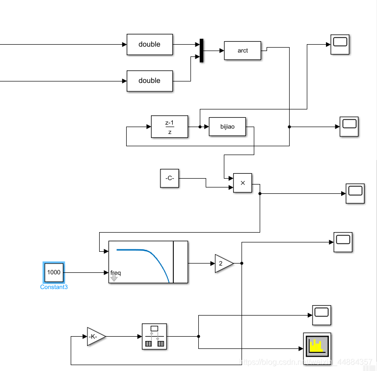
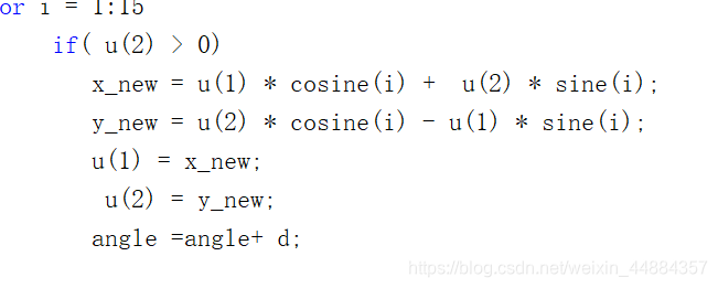
原理就是iq支路求一个arctan,得到瞬时角度,然后求导,得到瞬时频差。arctan也是自己写的s-function,用的cordic算法。这里注意输入有iq两个,要用mux模块换成一路。然后代码中,
iq两路信号是用u(1)、u(2)表示。
function [sys,x0,str,ts,simStateCompliance] = arct(t,x,u,flag)
%SFUNTMPL General MATLAB S-Function Template
% With MATLAB S-functions, you can define you own ordinary differential
% equations (ODEs), discrete system equations, and/or just about
% any type of algorithm to be used within a Simulink block diagram.
%
% The general form of an MATLAB S-function syntax is:
% [SYS,X0,STR,TS,SIMSTATECOMPLIANCE] = SFUNC(T,X,U,FLAG,P1,...,Pn)
%
% What is returned by SFUNC at a given point in time, T, depends on the
% value of the FLAG, the current state vector, X, and the current
% input vector, U.
%
% FLAG RESULT DESCRIPTION
% ----- ------ --------------------------------------------
% 0 [SIZES,X0,STR,TS] Initialization, return system sizes in SYS,
% initial state in X0, state ordering strings
% in STR, and sample times in TS.
% 1 DX Return continuous state derivatives in SYS.
% 2 DS Update discrete states SYS = X(n+1)
% 3 Y Return outputs in SYS.
% 4 TNEXT Return next time hit for variable step sample
% time in SYS.
% 5 Reserved for future (root finding).
% 9 [] Termination, perform any cleanup SYS=[].
%
%
% The state vectors, X and X0 consists of continuous states followed
% by discrete states.
%
% Optional parameters, P1,...,Pn can be provided to the S-function and
% used during any FLAG operation.
%
% When SFUNC is called with FLAG = 0, the following information
% should be returned:
%
% SYS(1) = Number of continuous states.
% SYS(2) = Number of discrete states.
% SYS(3) = Number of outputs.
% SYS(4) = Number of inputs.
% Any of the first four elements in SYS can be specified
% as -1 indicating that they are dynamically sized. The
% actual length for all other flags will be equal to the
% length of the input, U.
% SYS(5) = Reserved for root finding. Must be zero.
% SYS(6) = Direct feedthrough flag (1=yes, 0=no). The s-function
% has direct feedthrough if U is used during the FLAG=3
% call. Setting this to 0 is akin to making a promise that
% U will not be used during FLAG=3. If you break the promise
% then unpredictable results will occur.
% SYS(7) = Number of sample times. This is the number of rows in TS.
%
%
% X0 = Initial state conditions or [] if no states.
%
% STR = State ordering strings which is generally specified as [].
%
% TS = An m-by-2 matrix containing the sample time
% (period, offset) information. Where m = number of sample
% times. The ordering of the sample times must be:
%
% TS = [0 0, : Continuous sample time.
% 0 1, : Continuous, but fixed in minor step
% sample time.
% PERIOD OFFSET, : Discrete sample time where
% PERIOD > 0 & OFFSET < PERIOD.
% -2 0]; : Variable step discrete sample time
% where FLAG=4 is used to get time of
% next hit.
%
% There can be more than one sample time providing
% they are ordered such that they are monotonically
% increasing. Only the needed sample times should be
% specified in TS. When specifying more than one
% sample time, you must check for sample hits explicitly by
% seeing if
% abs(round((T-OFFSET)/PERIOD) - (T-OFFSET)/PERIOD)
% is within a specified tolerance, generally 1e-8. This
% tolerance is dependent upon your model's sampling times
% and simulation time.
%
% You can also specify that the sample time of the S-function
% is inherited from the driving block. For functions which
% change during minor steps, this is done by
% specifying SYS(7) = 1 and TS = [-1 0]. For functions which
% are held during minor steps, this is done by specifying
% SYS(7) = 1 and TS = [-1 1].
%
% SIMSTATECOMPLIANCE = Specifices how to handle this block when saving and
% restoring the complete simulation state of the
% model. The allowed values are: 'DefaultSimState',
% 'HasNoSimState' or 'DisallowSimState'. If this value
% is not speficified, then the block's compliance with
% simState feature is set to 'UknownSimState'.
% Copyright 1990-2010 The MathWorks, Inc.
%
% The following outlines the general structure of an S-function.
%
switch flag,
%%%%%%%%%%%%%%%%%%
% Initialization %
%%%%%%%%%%%%%%%%%%
case 0,
[sys,x0,str,ts,simStateCompliance]=mdlInitializeSizes;
%%%%%%%%%%%%%%%
% Derivatives %
%%%%%%%%%%%%%%%
case 1,
sys=mdlDerivatives(t,x,u);
%%%%%%%%%%
% Update %
%%%%%%%%%%
case 2,
sys=mdlUpdate(t,x,u);
%%%%%%%%%%%
% Outputs %
%%%%%%%%%%%
case 3,
sys=mdlOutputs(t,x,u);
%%%%%%%%%%%%%%%%%%%%%%%
% GetTimeOfNextVarHit %
%%%%%%%%%%%%%%%%%%%%%%%
case 4,
sys=mdlGetTimeOfNextVarHit(t,x,u);
%%%%%%%%%%%%%
% Terminate %
%%%%%%%%%%%%%
case 9,
sys=mdlTerminate(t,x,u);
%%%%%%%%%%%%%%%%%%%%
% Unexpected flags %
%%%%%%%%%%%%%%%%%%%%
otherwise
DAStudio.error('Simulink:blocks:unhandledFlag', num2str(flag));
end
% end sfuntmpl
%
%=============================================================================
% mdlInitializeSizes
% Return the sizes, initial conditions, and sample times for the S-function.
%=============================================================================
%
function [sys,x0,str,ts,simStateCompliance]=mdlInitializeSizes
%
% call simsizes for a sizes structure, fill it in and convert it to a
% sizes array.
%
% Note that in this example, the values are hard coded. This is not a
% recommended practice as the characteristics of the block are typically
% defined by the S-function parameters.
%
sizes = simsizes;
sizes.NumContStates = 0;
sizes.NumDiscStates = 0;
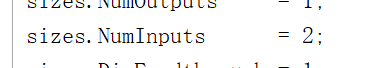
sizes.NumOutputs = 1;
sizes.NumInputs = 2;
sizes.DirFeedthrough = 1;
sizes.NumSampleTimes = 1; % at least one sample time is needed
sys = simsizes(sizes);
%
% initialize the initial conditions
%
x0 = [];
%
% str is always an empty matrix
%
str = [];
%
% initialize the array of sample times
%
ts = [-1 0];
% Specify the block simStateCompliance. The allowed values are:
% 'UnknownSimState', < The default setting; warn and assume DefaultSimState
% 'DefaultSimState', < Same sim state as a built-in block
% 'HasNoSimState', < No sim state
% 'DisallowSimState' < Error out when saving or restoring the model sim state
simStateCompliance = 'UnknownSimState';
end
%
%=============================================================================
% mdlDerivatives
% Return the derivatives for the continuous states.
%=============================================================================
%
function sys=mdlDerivatives(t,x,u)
sys = [];
end
%
%=============================================================================
% mdlUpdate
% Handle discrete state updates, sample time hits, and major time step
% requirements.
%=============================================================================
%
function sys=mdlUpdate(t,x,u)
sys = [];
end
%
%=============================================================================
% mdlOutputs
% Return the block outputs.
%=============================================================================
%
function sys=mdlOutputs(t,x,u)
sine=[ 0.7071067811865,0.3826834323651,0.1950903220161,0.09801714032956,...
0.04906767432742,0.02454122852291,0.01227153828572,0.006135884649154,...
0.003067956762966,0.001533980186285,7.669903187427045e-4,3.834951875713956e-4,...
1.917475973107033e-4,9.587379909597735e-5,4.793689960306688e-5,2.396844980841822e-5];
cosine =[0.7071067811865,0.9238795325113,0.9807852804032,0.9951847266722,...
0.9987954562052,0.9996988186962,0.9999247018391,0.9999811752826,...
0.9999952938096,0.9999988234517,0.9999997058629,0.9999999264657,...
0.9999999816164,0.9999999954041,0.999999998851,0.9999999997128];
d = 45.0;
angle = 0.0;
for i = 1:15
if( u(2) > 0)
x_new = u(1) * cosine(i) + u(2) * sine(i);
y_new = u(2) * cosine(i) - u(1) * sine(i);
u(1) = x_new;
u(2) = y_new;
angle =angle+ d;
else
x_new = u(1) * cosine(i) - u(2) * sine(i);
y_new = u(2) * cosine(i) + u(1) * sine(i);
u(1) = x_new;
u(2) = y_new;
angle =angle - d;
end
d =d / 2;
end
sys=angle;
end
%
%=============================================================================
% mdlGetTimeOfNextVarHit
% Return the time of the next hit for this block. Note that the result is
% absolute time. Note that this function is only used when you specify a
% variable discrete-time sample time [-2 0] in the sample time array in
% mdlInitializeSizes.
%=============================================================================
%
function sys=mdlGetTimeOfNextVarHit(t,x,u)
sampleTime = 1; % Example, set the next hit to be one second later.
sys = t + sampleTime;
end
%
%=============================================================================
% mdlTerminate
% Perform any end of simulation tasks.
%=============================================================================
%
function sys=mdlTerminate(t,x,u)
sys = [];
% end mdlTerminate
end
end
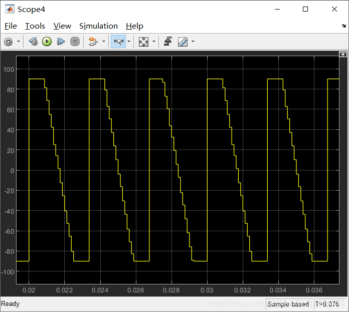
自己写的硬件能实现的artcan,在输入为无穷、输出为90°时,分辨率肯定很差,所以有一段平的,然后求导时,有一个90°到-90°的阶跃,要想办法去掉,也是自己写的一个s-function。
function sys=mdlOutputs(t,x,u)
if(u<-90  )
    sys=u+180;
else if(u>90  )
    sys=u-180;
    else sys=u;
    end
end
 end
当差值大于90°时,给一个180°的补偿。
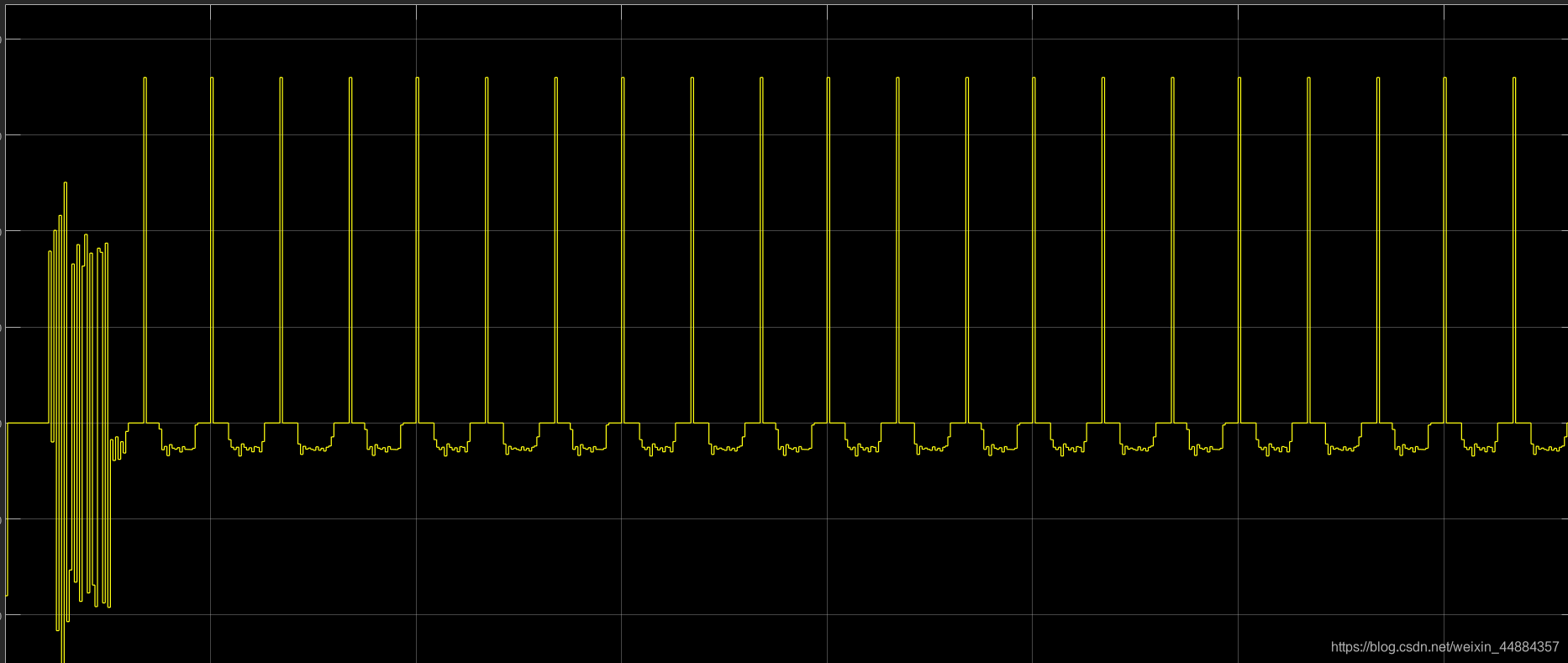
然后求导后:
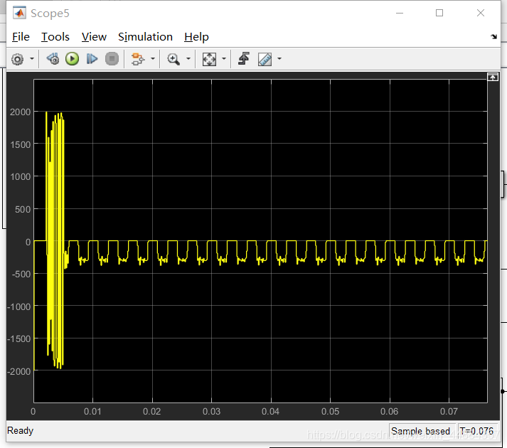
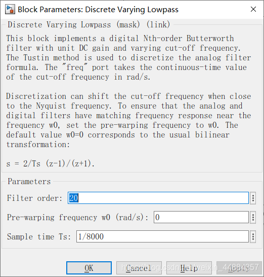
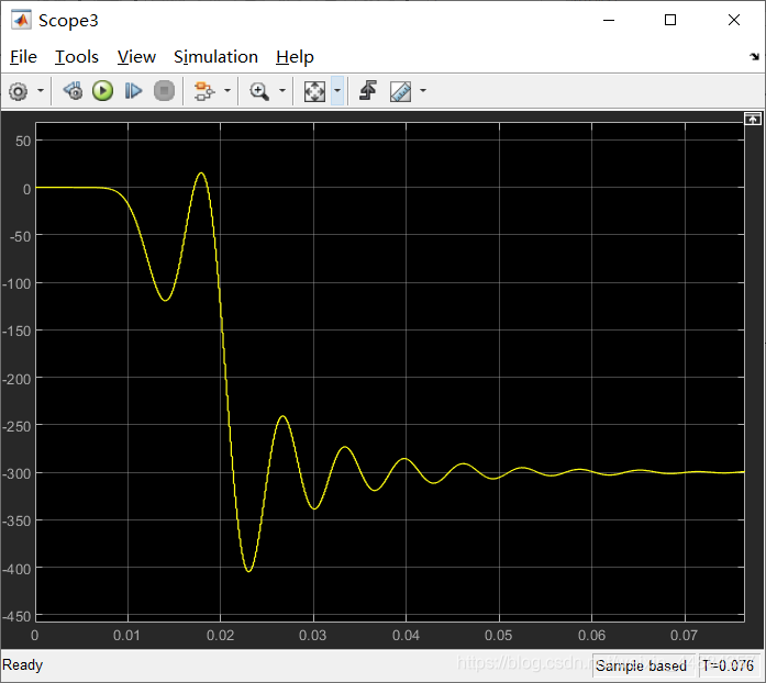
由于前面90°处分辨率不高的原因,求导后有一段是0,一段是频差交替出现。这里应该用环路滤波器什么的做处理吧。我不会,就只用了一个低通滤波器。
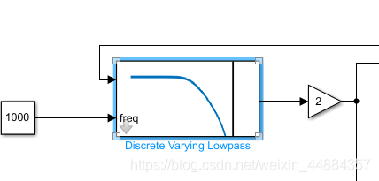
然后做一些倍数调整什么的,就能得到频差300Hz了.诶,还不错哦。
想用这个信号直接控制nco频率控制字调整本地载波,但是一直报错,做不出来,不管了。
就这了吧。


 987
987

 被折叠的 条评论
为什么被折叠?
被折叠的 条评论
为什么被折叠?
 到【灌水乐园】发言


