Transfer learning based multi-fidelity physics informed deep neural network论文笔记

论文信息

题目：Transfer learning based multi-fidelity physics informed deep neural network

作者：Souvik Chakraborty

期刊会议： Machine Learning (cs.LG); Computational Physics (physics.comp-ph)

年份：2020

论文地址：

代码：

基础补充

内容

动机

动机：

• 基于某些假设和近似，一些控制方程可以得到，但是建立的这个模型属于low-fidelity模型
• 通过实验，可以得到high-fidelity data，但是当数据收集昂贵且耗时，得到大量high-fidelity data 非常困难
• 同时利用low-fidelity模型与少量的high-fidelity data
• One possible solution to the difficulties raised above resides in multi-fidelity schemes where data fusion tech- niques are used to combine high-fidelity and low-fidelity data.

前人工作：

• The most popular multi-fidelity schemes are perhaps the multi-level Monte Carlo (MLMC) methods. MLMC fails when the low-fidelity and high-fidelity data have a space-dependent, complex and nonlinear correlations.
• The field of artificial intelligence and machine learning has recently witnessed a huge boom and its influence can also be observed in the multi-fidelity approaches. De et al ¹ developed two multi-fidelity approaches by using deep neural networks.
• While the first framework uses transfer learning, the second framework utilizes bi-fidelity weighted learning. Meng and Karniadakis ², on the other hand, proposed a composite neural network that is trained based on multi-fidelity data.

Based on the discussion above, (at least) two salient conclusions can be drawn about the existing multi-fidelity approaches:

• First, the existing multi-fidelity approaches assume the low-fidelity solver to be computationally efficient so that one can generate sufficient low-fidelity data.
• Second, the physics informed multi-fidelity approaches proposed in ³ assume that the exact physics cor- responding to the high-fidelity data is known. This is not necessarily true. There are problems where the underlying physics is unknown [1]. Also, the apparently known governing equations are often derived based on
  创新：

问题定义

The probability of failure of the system can be calculated as
$\begin{array}{rl}{P}_f=\mathbb{P}\left(\mathbf{\Xi }\in {\Omega }_f\right)& ={\int }_{{\Omega }_f}\mathrm{d}{F}_{\Xi }(\mathbf{\xi })\\ & ={\int }_{\Omega }{\mathbb{I}}_{{\Omega }_f}\mathrm{d}{F}_{\Xi }(\mathbf{\xi })\end{array}$
数据点的数量$N_h$意义重大,可以直接训练代理模型,$\mathcal{M}:(\xi ,x,t)\to u$然后用它来评估上式失败的概率

然而，在现实中，可以执行的实验室实验数量是有限的，因此，可用的数据点的数量往往不足以训练一个替代模型。为了补偿只有有限数量的高保真数据可用这一事实，我们考虑了系统的近似(低保真)控制方程:
${\mathbb{I}}_c(\mathbf{\xi })=\{\begin{array}{ll}1& \text{ if }\mathbf{\xi }\in c\\ 0& \text{ if }\mathbf{\xi }\notin c\end{array}$

$u_t+h\left(u,u_x,u_{xx},\dots ;\mathbf{\xi }\right)=0$

方法

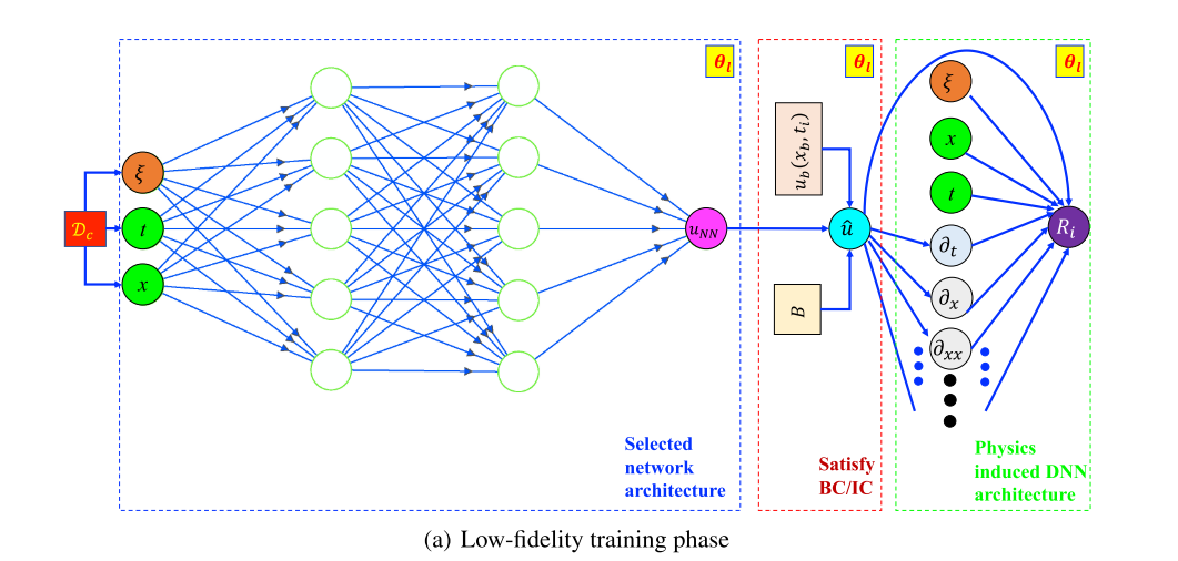
• 用常/偏微分方程给出了低逼真度模型，该模型不需要低保真度数据;相反，初始的低保真度模型直接训练基于问题的(近似)物理。这是通过利用最近开发的物理信息深度学习算法来实现的，通过这样的设置，一些重要的物理定律，比如低保真度模型中存在的不变性和对称性，将会被深度学习框架固有地捕捉到。
• 然后使用迁移学习和可用的高保真数据更新训练好的

Physics-informed deep neural networks

• 对于现在一些纯数据驱动的DNN来说，需要大量的高可信度的数据参与训练。然而，对于目前的这片paper工作来说，焦点集中在很少能获得高保真数据的问题上。因此，直接应用数据驱动的DNN不太可能产生令人满意的结果。所以，为了解决数据驱动的DNN对训练数据的过度依赖，PINN被提出。

• PINN有两个主要的优点：首先，与数据驱动的DNN等其他可靠性分析工具不同，PI-DNN不需要仿真数据。这将大大降低计算成本。其次，通过满足系统的控制微分方程来训练PI-DNN。因此，满足了不变性和对称性等物理特性。

• 但是对于PINN求解，准确的控制方程是已知的，但是在科学和工程中存在着许多控制微分方程⁴未知的情况。即使控制方程是已知的，它经常是基于某些假设和近似。

Proposed approach

3.1节中的数据驱动的DNN和3.2节中的PINN都不能解决第2节中定义的可靠性分析问题

• 数据驱动的DNN失败是因为高保真数据的数量，$N_h$非常少。另一方面，PI-DNN不能作为Eq.(7)中的控制微分方程，只能近似地表示实际情况。
• A multi-fidelity Aphysics informed deep neural network (MF-PIDNN) is presented in this section. MF-PIDNN utilizes the concepts of both data-driven and physics informed DNNs. Unlike available multi-fidelity frameworks, the proposed MF-PIDNN does not assume that generating low-fidelity data is trivial. In fact, no low-fidelity data is needed for the MF-PIDNN presented here.
• The key consideration of any multi-fidelity framework is associated with discovering and exploiting the relation be- tween the low-fidelity and high-fidelity model/data. In most of the frameworks available in the literature, this is achieved by using two surrogates; the first surrogate is trained based on the low-fidelity data and the second surrogate is used to find the functional relation between the low-fidelity and the high-fidelity data. This paper takes a separate route; instead of using two DNNs, a single DNN is first trained for the low-fidelity model and then updated based on the high-fidelity data.

方法：主要分成两步

• 第一步，使用PINN求解low-fidelity模型
• 第二步，然后用high-fidelity data${\mathcal{D}}_{hx}$更新low-fidelity模型(将low-fidelity模型网络参数作为初始化，用${\mathcal{D}}_{hx}$只更新最后一个或两个层对应的参数)

优势（使用了迁移学习）

• First, because of transfer learning, the number of parameters to be updated is reduced. This in turn, accelerates training of the DNN.
• Second, freezing the parameters of the initial layer ensures that the features learned/extracted from the low- fidelity model are retained in the network.
• Thirdly, transfer learning also ensures that the DNN does not overfit the high-fidelity data, Dh.

实验

our numerical examples are presented to illustrate the performance of the proposed approach. A wide variety of examples involving single and multiple stochastic variables, linear and non-linear problems, ordinary and partial differential equations are selected

实验1

$\frac{\mathrm{d}{u}_l}{\mathrm{d}t}=-Z{u}_l$
满足下面初值：
$u_l(t=0)=1.0$(21)
high-fidelity model：
$u_h=t\sin (t){\left[\log \left(u_l^4\right)\right]}^2+15t^3+1.0$(22)
The relation between the high-fidelity $u_h$ and the low-fidelity $u_l$ is non-linear. The limit-state function for this problem is defined as
$\mathcal{J}\left(Z,t_t\right)=u_h\left(Z,t_t\right)-u_0$ (23)

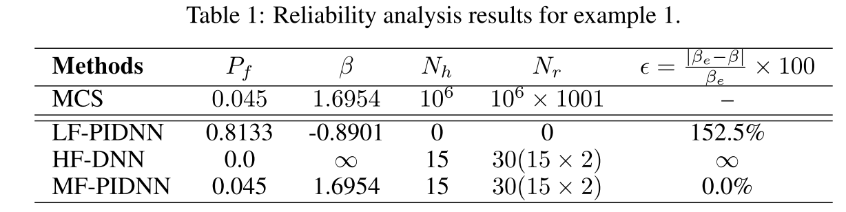
For this example, $t_t=1.0$ and $u_0=18.0$ is considered. It is assumed that 15 samples from the high- fidelity model is available,and for each of the 15 high-fidelity samples, the observations are available at t = [0.0, 1.0]. Note that the data-generation process, i.e., Eq. (23) is not known. MF-PIDNN only have access to the high-fidelity data and the low-fidelity model in Eq. (21).

Process:

• First step:
  $\hat{u}=t\cdot u_{N}N+1.0$
  The residual for training the low-fidelity DNN is
  $R_i=\frac{\mathrm{d}{\hat{u}}_i}{\mathrm{d}t}+Z_i{\hat{u}}_i$
• After training the physics-informed low-fidelity DNN, the next step is to update the model based on the high-fidelity data by using the transfer learning.

Table 1 shows the results obtained using MCS and MF-PIDNN

• The results obtained using MF-PIDNN matches exactly with the MCS results.
• To show the utility of the proposed approach, results obtained using only the low-fidelity PI-DNN and the high-fidelity DNN are also presented. Both low-fidelity PI-DNN and high-fidelity DNN are found to yield erroneous results.
  
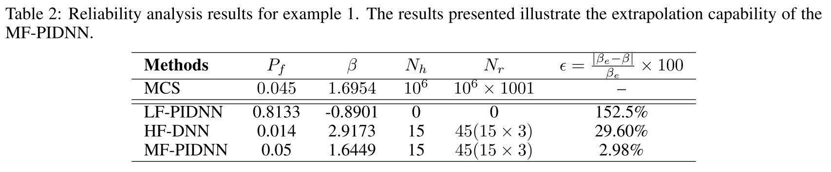
  To that end, it is assumed that for each of the 15 high-fidelity samples, observations are available t = [0.0, 0.5, 0.9], and the objective is to compute the reliability of the system at t = 1.0. The results obtained are shown in Table 2.
• Compared to the results presented in Table 1, slight deterioration in the results have been observed;This is expected because this is an extrapolation problem.
• Nonetheless, the results obtained are still significantly more accurate as compared to HF-DNN and LF-PIDNN.
  
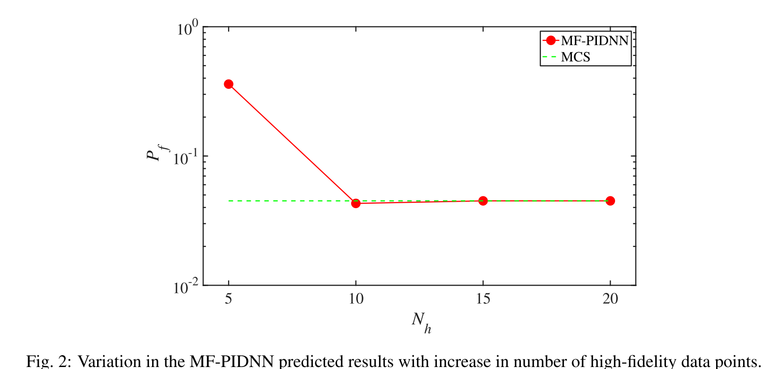
  Finally, the performance of the MF-PIDNN with variation in the number of high-fidelity data point, $N_h$ is investigated. For each realization of Z, the responses are observed at t = [0.0, 1.0] and the probability of failure at $t_t=1.0$ is computed. The variation of the MF-PIDNN predicted probability of failure is shown in Fig. 2.
• With an increase in $N_h$, the MF-PIDNN predicted probability of failure converges to the MCS solution.
• The HF-DNN results, up to $N_h=20$, yields erroneous results (not shown in Fig. 2). This is because, with only observations at two time-instants, the DNN fails to predict the trend of the limit-state function. MF-PIDNN, on the other hand, learns the trend from the physics of the problem and then update itself based on
  

实验2

The low-fidelity model, on the other hand, is considered to be
$${\left(u_l\right)}_t=\nu {\left(u_l\right)}_{xx}$$
The high-fidelity model for this problem is
$${\left(u_h\right)}_t+u_h{\left(u_h\right)}_x=\nu {\left(u_h\right)}_{x}x$$

The boundary and the initial conditions：

$$\begin{array}{c}{u}_h(t,x=-1)=1+\delta u_h(t,x=1)=-1\\ u_h(t=0,x)=-1+(1+x)\left(1+\frac{\delta }{2}\right)\end{array}$$

Process：

• $\hat{u}=u_h(t=0,x)+t(1-x)(1+x)u_{NN}$
  $${R_i={\left({\hat{u}}_t\right)}_i-\nu (\hat{u}{)}_{xx})}_i$$

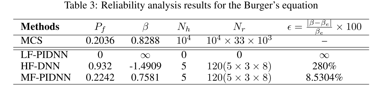
Along with MCS and MF-PIDNN results, LF-PIDNN and HF- DNN predicted results are also presented.

• Similar to the previous example, both probability of failure and reliability index are reported. It is observed that MF-PIDNN predicted results are extremely close to the MCS results.
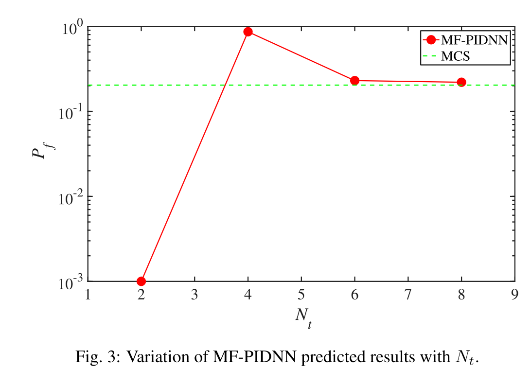
• HF- DNN and LF-PIDNN, on the other hand, yields erroneous results. Fig. 3 shows the performance of MF-PIDNN with increase in Nt (i.e, number of time-steps at which high-fidelity data is available).
  
  

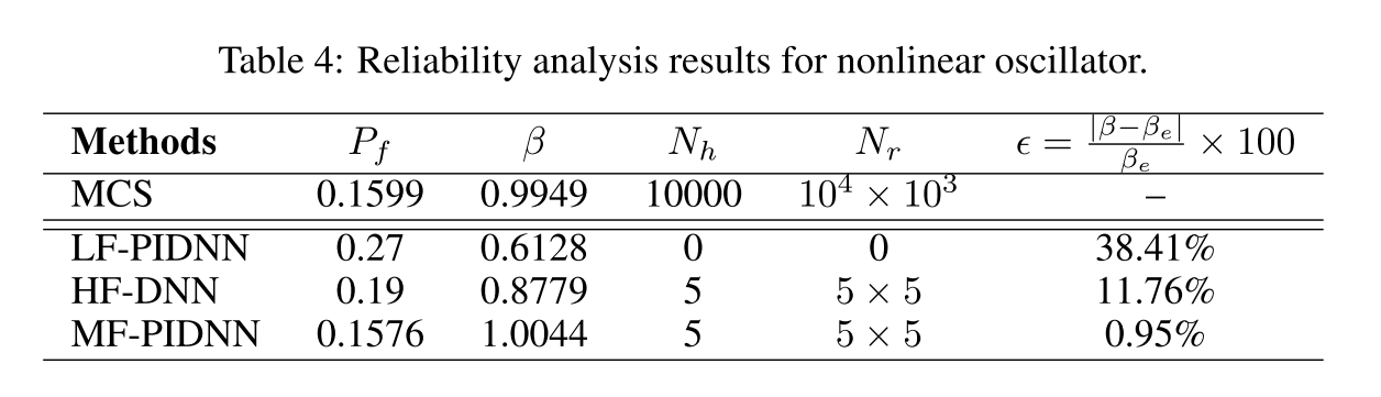
Nonlinear oscillator.

Methods
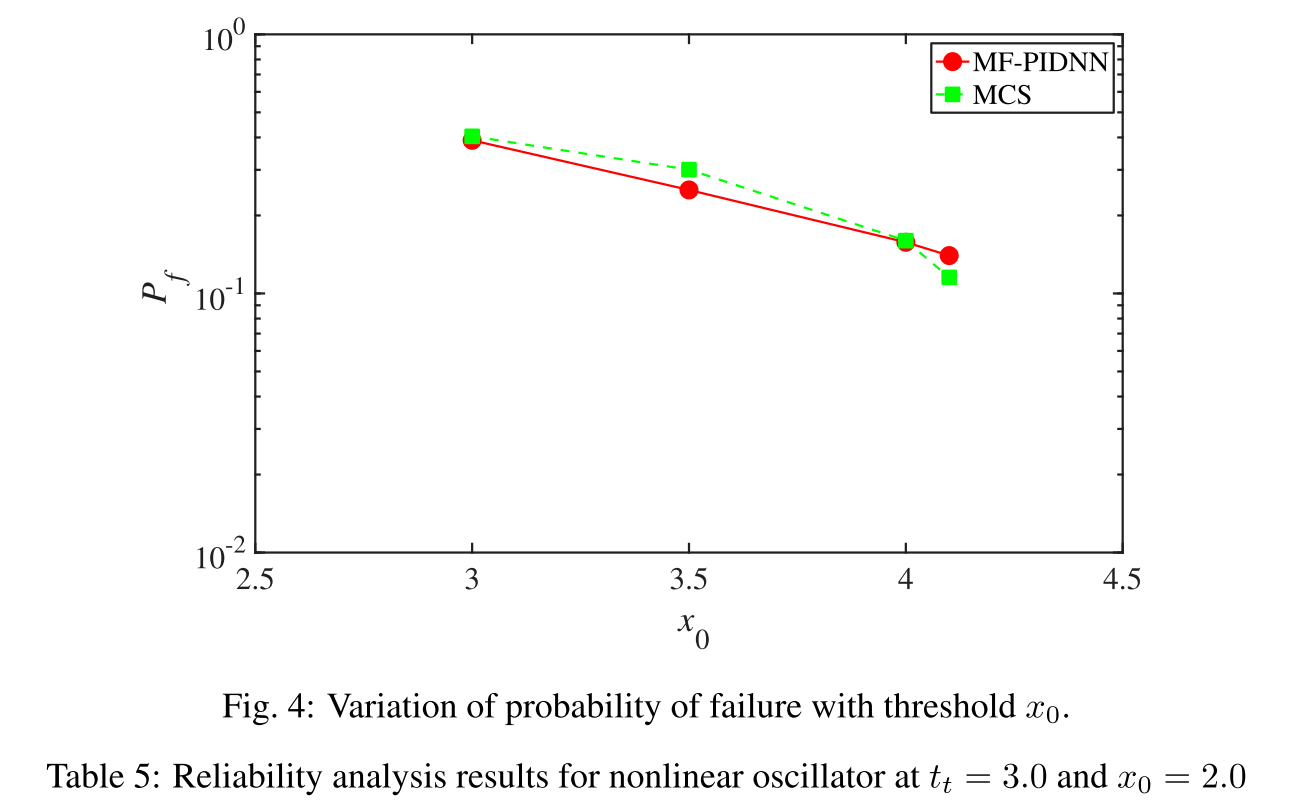
The variation of probability of failure with threshold x0 is shown in Fig. 4.

• Corresponding to all the thresholds, the MF-PIDNN predicted results matches closely with the MCS results. This indicates that the proposed MF-PIDNN is able to capture the response over the whole domain.
  
  

结论

In this paper, a multi-fidelity physics informed deep neural network (MF-PIDNN) is presented. The proposed approach is ideally suited for problems where the physics of the problem is known in an approximate sense (low-fidelity physics) and only a few high-fidelity data is available.

• MF-PIDNN blends the concepts of physics-informed and data-driven deep learning;
• The primary idea is to first train a low-fidelity deep learning model based on the available approximate physics and then use transfer learning to update the model based on the high-fidelity data.

There are two distinct advantages of MF-PIDNN.

• First, the low-fidelity model is directly trained from the physics of the problem and hence, no low-fidelity data is needed in this framework. - Second, because of the physics-informed framework within MF- PIDNN, the proposed approach is able to capture some of the physical laws that are present in the approximate model.

不足

不懂

可借鉴地方

---

1. Subhayan De, Jolene Britton, Matthew Reynolds, Ryan Skinner, Kenneth Jansen, and Alireza Doostan. On transfer learning of neural networks using bi-fidelity data for uncertainty propagation. arXiv preprint arXiv:2002.04495, 2020. ↩︎

2. Xuhui Meng and George Em Karniadakis. A composite neural network that learns from multi-fidelity data: Ap- plication to function approximation and inverse pde problems. Journal ofComputational Physics, 401:109020, 2020 ↩︎

3. Dehao Liu and Yan Wang. Multi-fidelity physics-constrained neural network and its application in materials modeling. Journal ofMechanical Design, 141(12), 2019. ↩︎

4. Steven L Brunton, Joshua L Proctor, and J Nathan Kutz. Discovering governing equations from data by sparse identification of nonlinear dynamical systems. Proceedings ofthe national academy ofsciences, 113(15):3932– 3937, 2016. ↩︎