《PyTorch深度学习实践》第五讲 用PyTorch实现线性回归

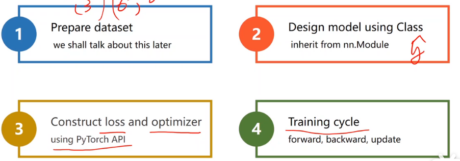
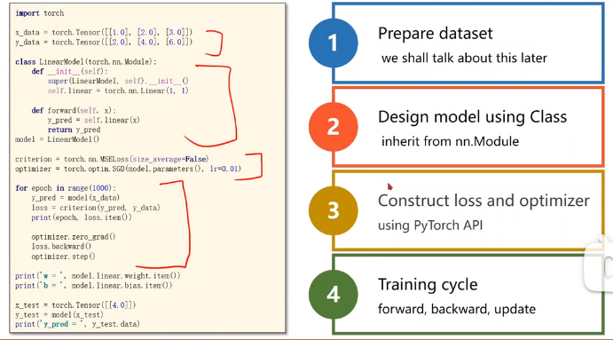
PyTorch Fashion（四步）

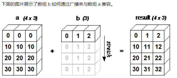
广播机制

numpy的广播机制： 广播(Broadcast)是 numpy 对不同形状(shape)的数组进行数值计算的方式。当运算中的 2 个数组的形状不同时，numpy 将自动触发广播机制。

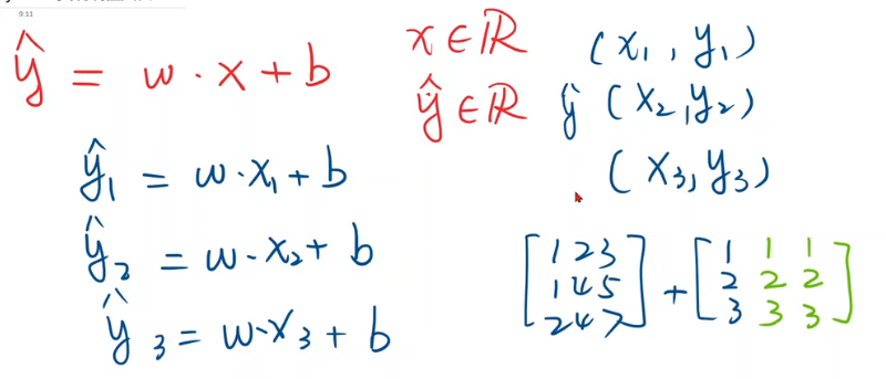
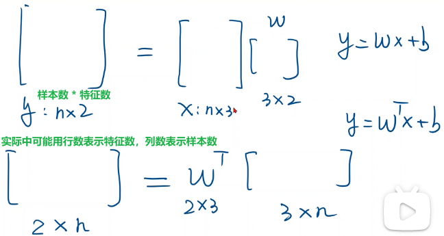
从前两节到现在的过渡，全写成向量形式

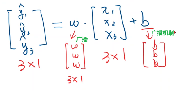
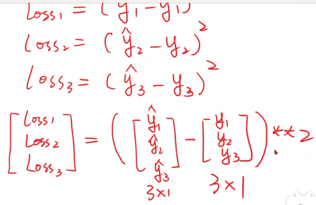
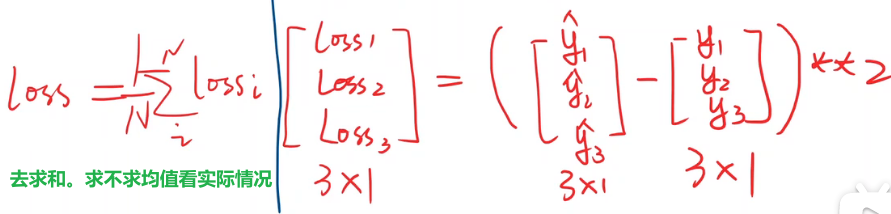
计算损失的过渡，全写成向量形式

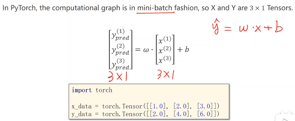
数据集准备

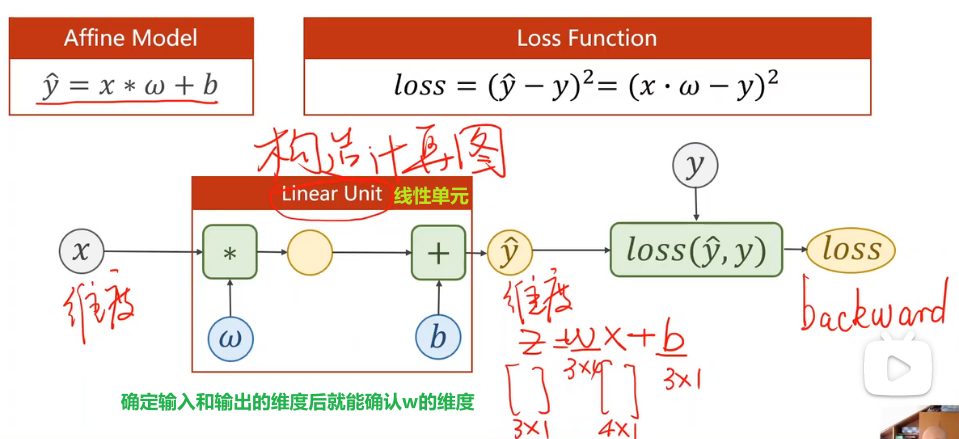
模型设计

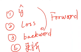
不需要人工求导数，重点的目标变成构造计算图

最终的loss必须是标量，才能使用loss.backward

代码分析

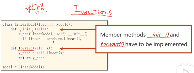
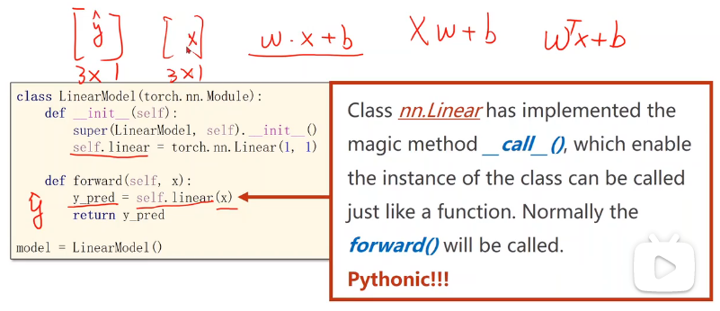
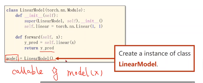
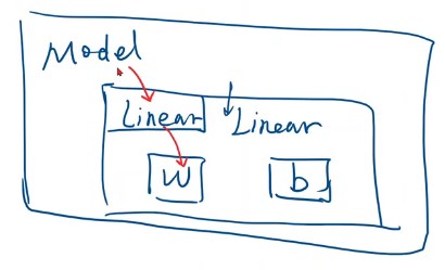
• 把模型定义成一个类，之后基本都是这个形式。必须掌握，将来可以扩展该模型使其适用于不同的任务。

• 这个类要继承自nn.Module，因为该父类中有很多方法，这些方法在模型训练过程中需要用到。

• 这个类中最少需要两个函数

1. __init__：构造函数，初始化对象时默认调用的函数

1. super：调用父类的构造，不用管，照着写。第一个参数是我们定义的类的名称

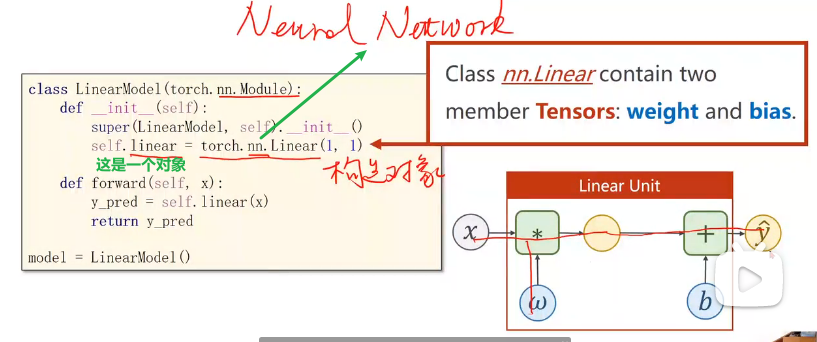
2. nn.Linear是一个类，包含两个成员张量：权重和偏置。类名（）：就是在构造对象。这个Linear也是继承自Module，所以可以自动进行反向传播

2. forward：前馈过程中需要执行的计算

1. 线性的计算块儿。直接在对象后面加（）， 这意味着实现了一个callable（可调用的对象）。在pytorch中，module的call里中的一个重要语句就是去调用forward。所以在我们的module中必须要实现forward函数。我们这里写的其实是函数的override，覆盖掉父类的forward。此处送进去x，其实是在算wx+b

• 不需要写backward是因为用module构造出来的对象会自动根据计算图实现backward的过程。如果我们需要的计算模块能由现成的pytorch的计算模块构成，用module确实是最简单的。（不需要人工设计反向传播的导数）

如果以后要用的一些模块在pytorch中没有定义，换句话说它没办法对其求导数。此时有两种方法能解决：

1. 如果你的模块能由基本的Python支持的运算来构成，你可以将其封装成一个model，将来去实例化并调用该model，它可以自动进行反向传播

2. 如果你感觉pytorch的计算图算起来效率不高，在计算导数时你有更高效的方法，那么可以从Functions中继承。Functions也是pytorch中的一个类，在该类中需要实现反向传播，可以构造自己的计算块

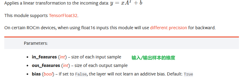
Linear — PyTorch 2.0 documentation

定义模型时直接这么写！记得由于它继承了那些，所以也是callable的

补充知识：位置参数，关键字参数

class Foobar:
    def __init__(self):
        pass

    def __call__(self,*args,**kwargs):# *args:位置参数，**kwargs：关键字参数
        print("hello " + str(args)) #必须转成字符串，can only concatenate str (not "tuple") to str
        print("hi " + str(kwargs))
    
f = Foobar()
f(1,2,3,c=10,d=100)

def func(*args,**kwargs):
    print("hello ",args) # 变成元组存起来
    print("hi ",kwargs) # 变成字典存起来

func(2,4,7,8,0,x=1,y=90)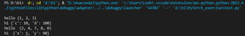

构造损失函数和优化器

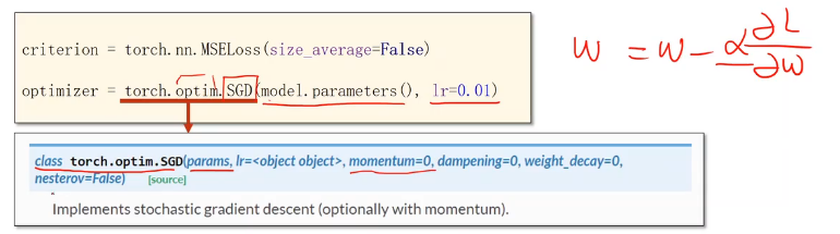
损失函数

nn.MSELoss也是继承自nn.Module

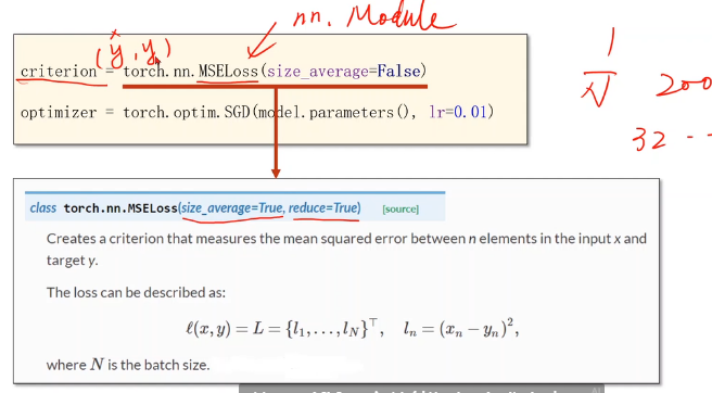
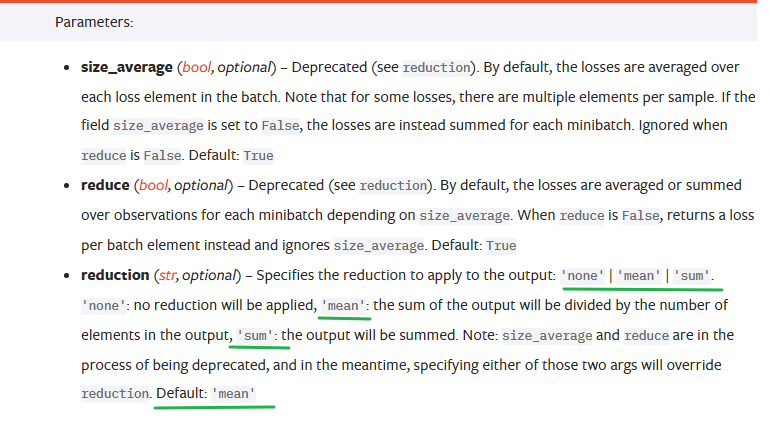
官方文档已经更新了，把两个参数合二为一并为一个参数了

优化器

torch.optim.SGD与torch.nn.Module无关，不参与构建计算图。

优化模块中有一个类叫做SGD，在此将其实例化

• model.parameters()：module模块中有个成员函数叫parameters，该函数会检查module中的所有成员，如果这些成员中有相应的权重，它就会把这些都加到最后要进行训练的参数集合上

在取得linear权重时调用了linear.parameters()

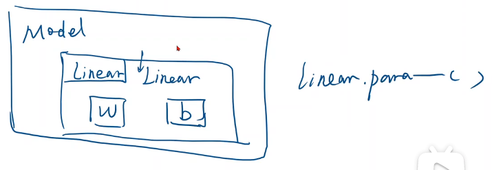
以后定义模型时经常会嵌套，比如在卷积神经网络模型中，用了很多inception计算块，每个inception中又包含了很多可训练的计算块，parameters这个函数能用类似递归的方式把模型里涉及到的要训练的权重全找出来

• lr = 0.01：pytorch还支持在模型的不同部分（即权重更新公式）使用不同的学习率

训练过程

注意在print loss时，其实loss是对象，它会自动调用__str__()函数变成标量，不会产生计算图。

写成loss.item()也行

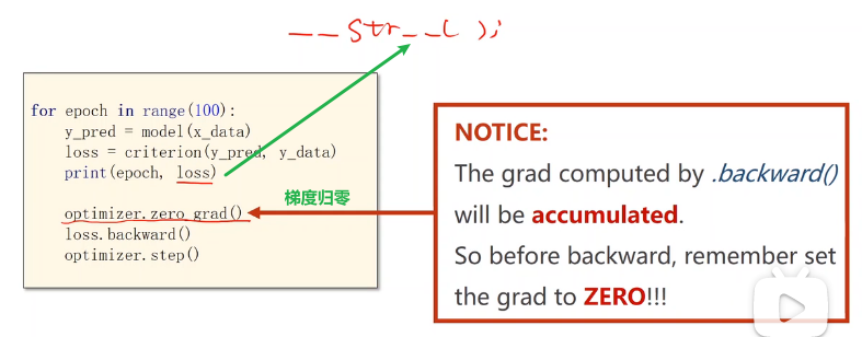
step()函数：进行一次更新，会根据所有参数里包含的梯度以及预先设计的学习率来自动进行更新

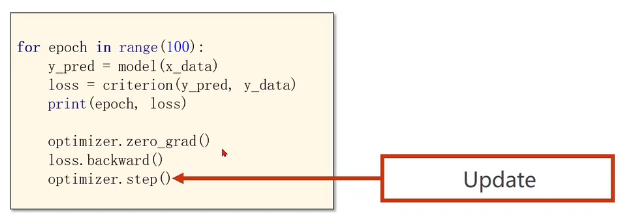
训练步骤总结

输出并测试模型

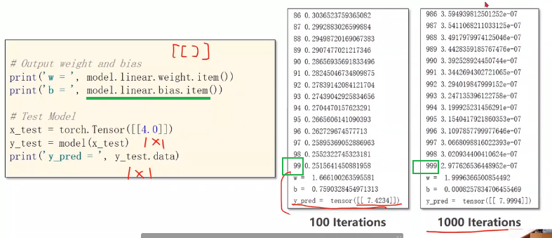
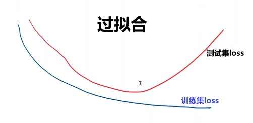
增加训练次数后预测值接近了我们想要的结果，但要注意防止过拟合。

总结

代码

import torch
import matplotlib.pyplot as plt
# prepare dataset
# x,y是矩阵，3行1列 也就是说总共有3个数据，每个数据只有1个特征
x_data = torch.tensor([[1.0], [2.0], [3.0]])
y_data = torch.tensor([[2.0], [4.0], [6.0]])
 
#design model using class
"""
our model class should be inherit from nn.Module, which is base class for all neural network modules.
member methods __init__() and forward() have to be implemented
class nn.linear contain two member Tensors: weight and bias
class nn.Linear has implemented the magic method __call__(),which enable the instance of the class can
be called just like a function.Normally the forward() will be called 
"""
class LinearModel(torch.nn.Module):
    def __init__(self):
        super(LinearModel, self).__init__()
        # (1,1)是指输入x和输出y的特征维度，这里数据集中的x和y的特征都是1维的
        # 该线性层需要学习的参数是w和b  获取w/b的方式分别是~linear.weight/linear.bias
        self.linear = torch.nn.Linear(1, 1)
 
    def forward(self, x):
        y_pred = self.linear(x)
        return y_pred
 
model = LinearModel()
 
# construct loss and optimizer
criterion = torch.nn.MSELoss(reduction = 'sum')
optimizer = torch.optim.SGD(model.parameters(), lr = 0.01) # model.parameters()自动完成参数的初始化操作
# optimizer=torch.optim.Adagrad(model.parameters(),lr=0.01)
# optimizer=torch.optim.Adam(model.parameters(),lr=0.01)
# optimizer=torch.optim.Adamax(model.parameters(),lr=0.01)
# optimizer=torch.optim.ASGD(model.parameters(),lr=0.01)
# optimizer=torch.optim.LBFGS(model.parameters(),lr=0.01) # step() missing 1 required positional argument: 'closure'
# optimizer=torch.optim.RMSprop(model.parameters(),lr=0.01)
# optimizer=torch.optim.Rprop(model.parameters(),lr=0.01)
# optimizer=torch.optim.Adadelta(model.parameters(),lr=0.01)

epoch_list = [] # 存起来好画图
loss_list = []

# training cycle forward, backward, update
for epoch in range(100):
    y_pred = model(x_data) # forward:predict
    loss = criterion(y_pred, y_data) # forward: loss
    print(epoch, loss.item())

    epoch_list.append(epoch)
    loss_list.append(loss.item())

    optimizer.zero_grad() # the grad computer by .backward() will be accumulated. so before backward, remember set the grad to zero
    loss.backward() # backward: autograd，自动计算梯度
    optimizer.step() # update 参数，即更新w和b的值
    print('\t', model.linear.weight.item(), model.linear.bias.item())

 
print('w = ', model.linear.weight.item())
print('b = ', model.linear.bias.item())

x_test = torch.tensor([[4.0]])
y_test = model(x_test)
print('y_pred = ', y_test.data)

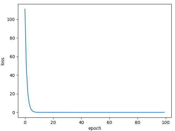
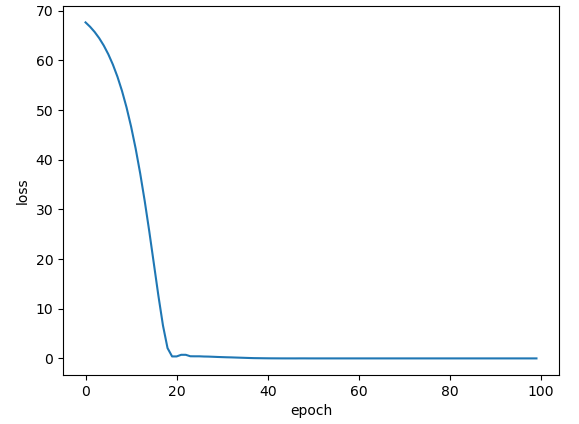
plt.figure(1)
plt.plot(epoch_list,loss_list)#画在图1上
plt.ylabel('loss')
plt.xlabel('epoch')
plt.show() 

参考：PyTorch 深度学习实践 第5讲_criterion = torch.nn.mseloss()_错错莫的博客-CSDN博客

对w b不需要附初始值，每次的初始值也都不一样

7、本实例是批量数据处理，小伙伴们不要被optimizer = torch.optim.SGD(model.parameters(), lr = 0.01)误导了，以为见了SGD就是随机梯度下降。要看传进来的数据是单个的还是批量的。这里的x_data是3个数据，是一个batch，调用的PyTorch API是 torch.optim.SGD，但这里的SGD不是随机梯度下降，而是批量梯度下降。也就是说，梯度下降算法使用的是随机梯度下降，还是批量梯度下降，还是mini-batch梯度下降，用的API都是 torch.optim.SGD。

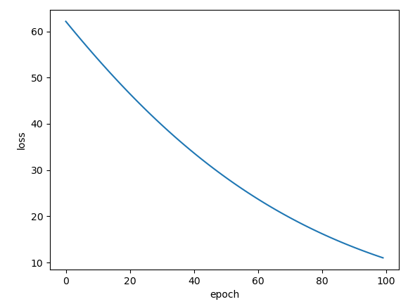
作业：

批量梯度下降SGD：

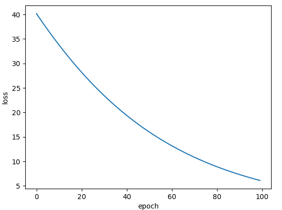
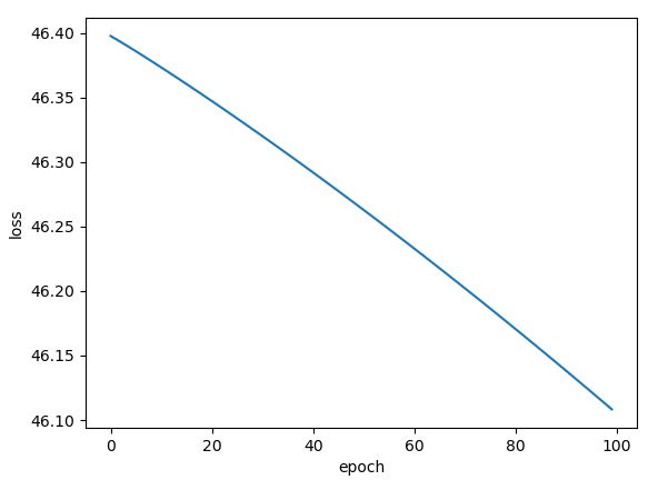
Adagrad:

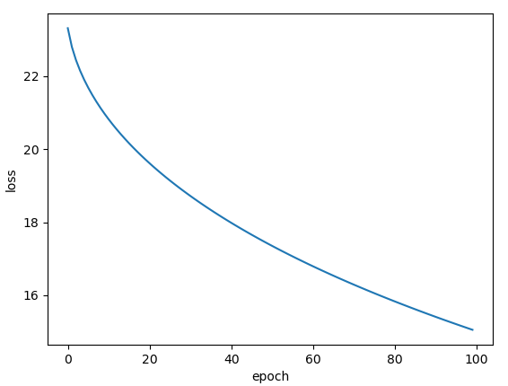
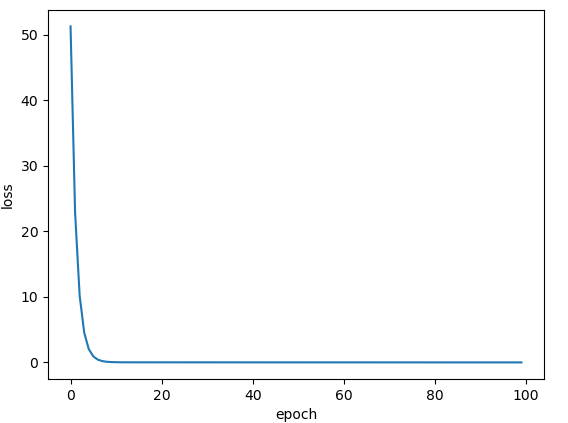
Adam:

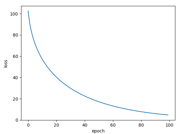
Adamax:

ASGD:

RMSprop:

Rprop:

Adadelta: