跟着Molecular Cancer学作图 -- 分半小提琴图

从这个系列开始，师兄就带着大家从各大顶级期刊中的Figuer入手，从仿照别人的作图风格到最后实现自己游刃有余的套用在自己的分析数据上！这一系列绝对是高质量！还不赶紧点赞+在看，学起来！

话不多说，直接上图！

示例数据和代码获取

生信常用分析图形+跟着高分SCI学作图

读图

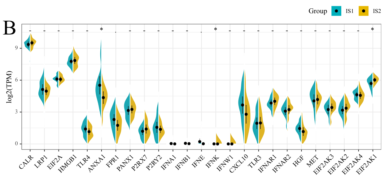
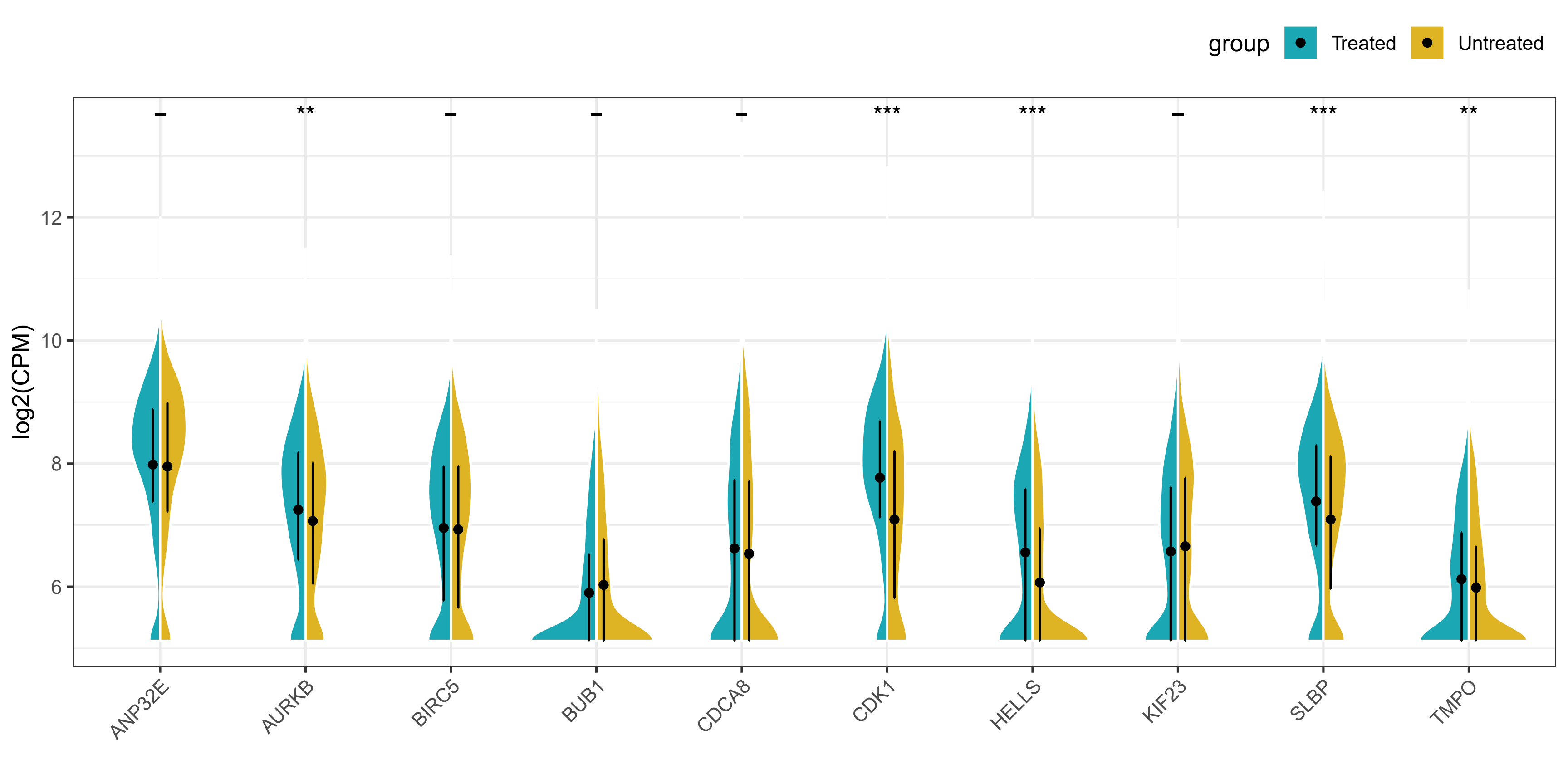
这张图理解起来没什么复杂的，就是一个分组提琴图，然后将两个组的小提琴分别显示一半，这样更方便读者直观比较。本小节我们介绍两种实现方法，一种是基于gghalves包中的geom_half_violin函数，另一种是借助github大佬编写的geom_split_violin函数。

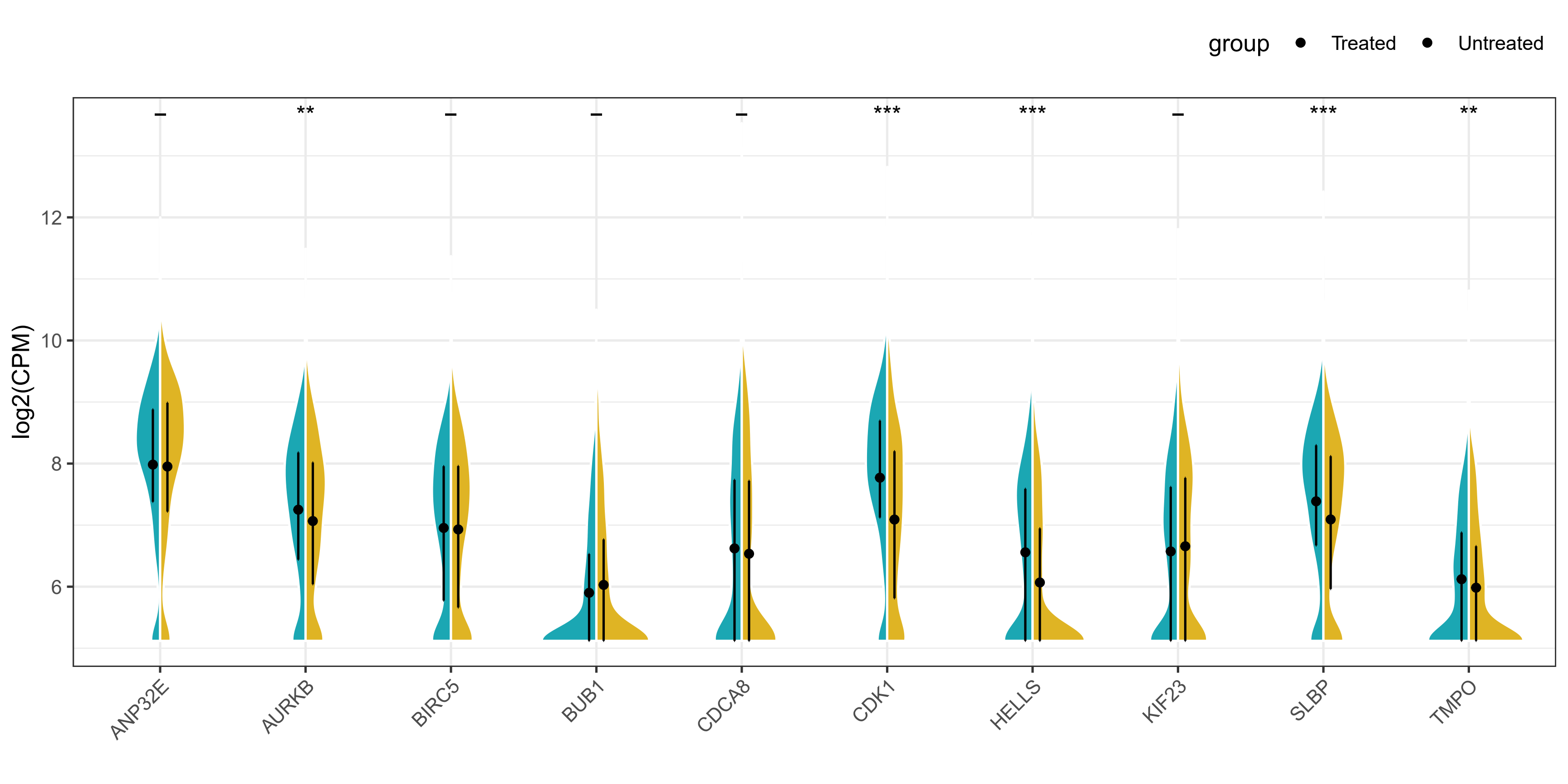
效果展示

由于本次使用的数据分布并不是很好，所以提琴的形状并不是很美观，但是图形的外观和细节都基本复现了原文。本次复现完全在R语言中进行，请大家放心食用！

数据构建

####################### 分半提琴图 ####################
library(ggplot2)
library(gghalves)
library(tidyverse)

# 读取测试数据：此数据集来源于GSE142651，随机挑选25个基因：
data <- read.csv("data.csv")
data <- data[sample(1:nrow(data), 10),]


# 宽数据转长数据：
data_new <- data %>% 
  pivot_longer(cols = !X, 
               names_to = "Samples", 
               values_to = "Values")

colnames(data_new)[1] <- "Genes"

# 添加分组信息：
data_new$group <- str_split(data_new$Samples, "_", simplify = T)[,4]
# 查看数据
head(data_new)
# # A tibble: 6 x 4
# Genes Samples                     Values group    
# <chr> <chr>                        <dbl> <chr>    
# 1 MCM5  Chip91481_r20_c71_Untreated   7.84 Untreated
# 2 MCM5  Chip91481_r47_c21_Untreated   5.12 Untreated
# 3 MCM5  Chip91484_r0_c62_Untreated    5.67 Untreated
# 4 MCM5  Chip91481_r16_c70_Untreated   5.12 Untreated
# 5 MCM5  Chip91484_r0_c35_Treated      6.67 Treated  
# 6 MCM5  Chip91484_r37_c38_Untreated   5.12 Untreated

绘图代码

geom_half_violin函数

# 绘图：
ggplot()+
  geom_half_violin(
    data = data_new %>% filter(group == "Treated"),
    aes(x = Genes,y = Values),colour="white",fill="#1ba7b3",side = "l"
  )+
  geom_half_violin(
    data = data_new %>% filter(group == "Untreated"),
    aes(x = Genes,y = Values),colour="white",fill="#dfb424",side = "r"
  )+
  theme_bw()+
  xlab("")+
  ylab("log2(CPM)")+
  geom_point(data = data_new, aes(x = Genes,y = Values, fill = group),
             stat = 'summary', fun=mean,
             position = position_dodge(width = 0.2))+
  stat_summary(data = data_new, aes(x = Genes,y = Values, fill = group),
               fun.min = function(x){quantile(x)[2]},
               fun.max = function(x){quantile(x)[4]},
               geom = 'errorbar', color='black',
               width=0.01,size=0.5,
               position = position_dodge(width = 0.2))+
  stat_compare_means(data = data_new, aes(x = Genes,y = Values, fill = group),
                     # 修改显著性标注：
                     symnum.args=list(cutpoints = c(0, 0.001, 0.01, 0.05, 1),
                                      symbols = c("***", "**", "*", "-")),
                     label = "p.signif",
                     label.y = max(data_new$Values),
                     hide.ns = F)+
  theme(axis.text.x = element_text(angle = 45, hjust = 1), 
        legend.position = "top",
        legend.justification = "right")
  

ggsave("violin_plot.pdf", height = 5, width = 10)

方法二

# 方法二：使用geom_split_violion函数：
# 函数来源：https://github.com/tidyverse/ggplot2/blob/eecc450f7f13c5144069705ef22feefe0b8f53f7/R/geom-violin.r#L102
GeomSplitViolin <- ggproto("GeomSplitViolin", GeomViolin, 
                           draw_group = function(self, data, ..., draw_quantiles = NULL) {
                             data <- transform(data, xminv = x - violinwidth * (x - xmin), xmaxv = x + violinwidth * (xmax - x))
                             grp <- data[1, "group"]
                             newdata <- plyr::arrange(transform(data, x = if (grp %% 2 == 1) xminv else xmaxv), if (grp %% 2 == 1) y else -y)
                             newdata <- rbind(newdata[1, ], newdata, newdata[nrow(newdata), ], newdata[1, ])
                             newdata[c(1, nrow(newdata) - 1, nrow(newdata)), "x"] <- round(newdata[1, "x"])
                             
                             if (length(draw_quantiles) > 0 & !scales::zero_range(range(data$y))) {
                               stopifnot(all(draw_quantiles >= 0), all(draw_quantiles <=
                                                                         1))
                               quantiles <- ggplot2:::create_quantile_segment_frame(data, draw_quantiles)
                               aesthetics <- data[rep(1, nrow(quantiles)), setdiff(names(data), c("x", "y")), drop = FALSE]
                               aesthetics$alpha <- rep(1, nrow(quantiles))
                               both <- cbind(quantiles, aesthetics)
                               quantile_grob <- GeomPath$draw_panel(both, ...)
                               ggplot2:::ggname("geom_split_violin", grid::grobTree(GeomPolygon$draw_panel(newdata, ...), quantile_grob))
                             }
                             else {
                               ggplot2:::ggname("geom_split_violin", GeomPolygon$draw_panel(newdata, ...))
                             }
                           })

geom_split_violin <- function(mapping = NULL, data = NULL, stat = "ydensity", position = "identity", ..., 
                              draw_quantiles = NULL, trim = TRUE, scale = "area", na.rm = FALSE, 
                              show.legend = NA, inherit.aes = TRUE) {
  layer(data = data, mapping = mapping, stat = stat, geom = GeomSplitViolin, 
        position = position, show.legend = show.legend, inherit.aes = inherit.aes, 
        params = list(trim = trim, scale = scale, draw_quantiles = draw_quantiles, na.rm = na.rm, ...))
}

ggplot(data_new, aes(x = Genes,y = Values, fill = group))+
  geom_split_violin(trim = T,colour="white")+
  geom_point(stat = 'summary',fun=mean,
             position = position_dodge(width = 0.2))+
  scale_fill_manual(values = c("#1ba7b3","#dfb424"))+
  stat_summary(fun.min = function(x){quantile(x)[2]},
               fun.max = function(x){quantile(x)[4]},
               geom = 'errorbar',color='black',
               width=0.01,size=0.5,
               position = position_dodge(width = 0.2))+
  stat_compare_means(data = data_new, aes(x = Genes,y = Values),
                     # 修改显著性标注：
                     symnum.args=list(cutpoints = c(0, 0.001, 0.01, 0.05, 1),
                                      symbols = c("***", "**", "*", "-")),
                     label = "p.signif",
                     label.y = max(data_new$Values),
                     hide.ns = F)+
  theme_bw()+
  xlab("")+
  ylab("log2(CPM)")+
  theme(axis.text.x = element_text(angle = 45, hjust = 1), 
        legend.position = "top",
        #legend.key = element_rect(fill = c("#1ba7b3","#dfb424")),
        legend.justification = "right")

ggsave("violin_plot2.pdf", height = 5, width = 10)

结果展示

示例数据和代码获取

生信常用分析图形+跟着高分SCI学作图

以上就是本期的全部内容啦！**欢迎点赞，点在看！**师兄会尽快更新哦！制作不易，你的打赏将成为师兄继续更新的十足动力！

往期文章

1. 跟着Nature Medicine学作图–箱线图+散点图
2. 跟着Nature Communications学作图–渐变火山图
3. 跟着Nature Communications学作图–气泡图+相关性热图
4. 跟着Nature Communications学作图 – 复杂提琴图
5. 跟着Nature Medicine学作图–复杂热图
6. 跟着Nature Communications学作图–复杂散点图
7. 跟着Nature Communications学作图 – 复杂百分比柱状图