


观看了吴恩达老师的深度学习公开课,总结了部分个人觉得有益的知识点。
一、数据结构
当编写神经网络程序时,就不要用这种秩为1的数据结构,如shape等于(n, ),或者是一维数组时。
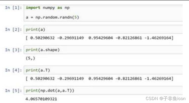
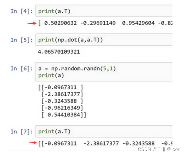
两对方括号和一对方括号,这就是1行5列的矩阵和一维数组的差别。

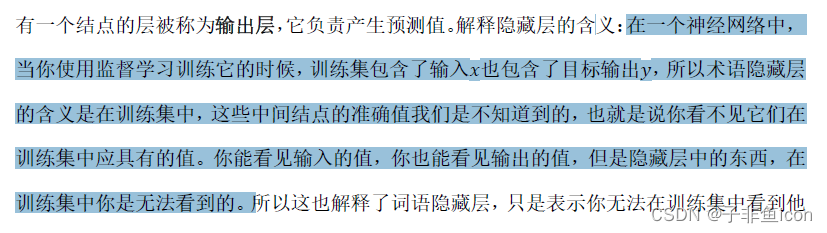
二.隐藏层的含义
三、L1W2作业
3.1 作业代码
import numpy as np
import matplotlib.pyplot as plt
import h5py
import scipy
from PIL import Image
from scipy import ndimage
from lr_utils import load_dataset
# load data
train_set_x_orig, train_set_y, test_set_x_orig, test_set_y, classes = load_dataset()
# 图片预览
index = 2
print(train_set_x_orig[index].shape)
plt.imshow(train_set_x_orig[index])
plt.show()
#打印出当前的训练标签值
#使用np.squeeze的目的是压缩维度,【未压缩】train_set_y[:,index]的值为[1] , 【压缩后】np.squeeze(train_set_y[:,index])的值为1
#print("【使用np.squeeze:" + str(np.squeeze(train_set_y[:,index])) + ",不使用np.squeeze: " + str(train_set_y[:,index]) + "】")
#只有压缩后的值才能进行解码操作
print("y=" + str(train_set_y[:,index]) + ", it's a '" + classes[np.squeeze(train_set_y[:,index])].decode("utf-8") + "' picture")
# 获取数据维度信息
print(train_set_x_orig.shape) # (209, 64, 64, 3)
print(train_set_y.shape) # (1, 209)
print(test_set_x_orig.shape) # (50, 64, 64, 3)
print(test_set_y.shape) # (1, 50)
m_train = train_set_y.shape[1]
m_test = test_set_y.shape[1]
num_px = test_set_x_orig.shape[1]
print("训练集的样本数:"+str(m_train))
print("测试集的样本数:"+str(m_test))
print("图片的宽和高:"+str(num_px))
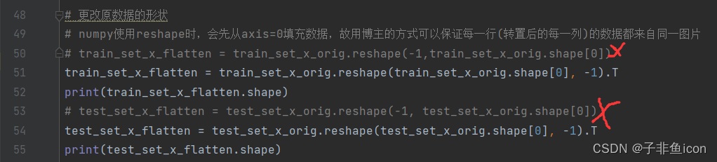
# 更改原数据的形状
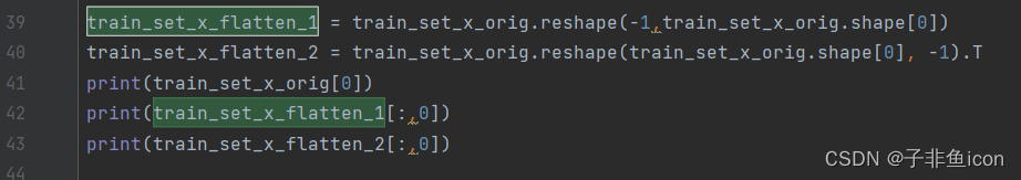
# numpy使用reshape时,会先从axis=0填充数据,故用博主的方式可以保证每一行(转置后的每一列)的数据都来自同一图片
# train_set_x_flatten = train_set_x_orig.reshape(-1,train_set_x_orig.shape[0])
train_set_x_flatten = train_set_x_orig.reshape(train_set_x_orig.shape[0], -1).T
print(train_set_x_flatten.shape)
# test_set_x_flatten = test_set_x_orig.reshape(-1, test_set_x_orig.shape[0])
test_set_x_flatten = test_set_x_orig.reshape(test_set_x_orig.shape[0], -1).T
print(test_set_x_flatten.shape)
# 标准化数据集
train_set_x = train_set_x_flatten /255
test_set_x = test_set_x_flatten /255
# 定义激活函数
def sigmoid(z):
s = 1/(1+np.exp(-z))
return s
# 初始化模型参数
def initialize_params(dim):
#W = np.random.normal(0,0.01,(train_set_x.shape[0],1))
#b = np.zeros((1,m_train))
W = np.zeros((dim, 1))
b = 0
# 使用断言确保数据正确
assert(W.shape == (dim, 1))
assert(isinstance(b, float) or isinstance(b, int))
return W, b
# 传播函数
def propagate(W, b, X, y):
m = X.shape[1]
# 正向传播
Z = np.dot(W.T, X) + b
A = sigmoid(Z)
J = np.sum(-y*np.log(A)-(1-y)*np.log(1-A))/m
# 反向传播
dZ = A - y
dw = np.dot(X, dZ.T) / m
db = np.sum(dZ) / m
grads = {"dw": dw, "db": db} #用字典来保存
return J, grads
# 更新参数
def optimizer(W, b, X, y, num_iterations, lr, show_cost):
cost_ls = []
for i in range(num_iterations):
cost, grads = propagate(W, b, X, y)
dw = grads["dw"]
db = grads["db"]
W = W - lr*dw
b = b - lr*db
if i % 100 == 0:
cost_ls.append(cost)
if(show_cost) and (i % 100 == 0):
print(i,"----->",cost)
params = {"W":W, "b":b}
grads = {"dw": dw, "db": db}
return params, grads, cost_ls
# 预测函数
def predict(W, b, X):
m = X.shape[1]
A = sigmoid(np.dot(W.T, X) + b)
y_pred = np.zeros((1, m))
for i in range(A.shape[1]):
y_pred[0, i] = 1 if A[0, i] >= 0.5 else 0
return y_pred
# 整合成一个函数
def model(X_train, y_train, X_test, y_test, num_iterations=2000, lr=0.5, show_cost=False): # 学习率设置过大,或导致内存溢出,出现nan
W, b = initialize_params(X_train.shape[0])
params, grads, cost_ls = optimizer(W, b, X_train, y_train, num_iterations, lr, show_cost)
W = params["W"]
b = params["b"]
y_pred_train = predict(W, b, X_train)
y_pred_test = predict(W, b, X_test)
print("训练集准确性:", format(100-np.mean(np.abs(y_pred_train - y_train))*100),"%") # 相同为0,不同为1
print("测试集准确性:", format(100 - np.mean(np.abs(y_pred_test - y_test)) * 100), "%")
d = {"cost_ls":cost_ls,"y_pred_train":y_pred_train, "y_pred_test":y_pred_test, "W":W, "b":b, "lr":lr}
return d
d = model(train_set_x, train_set_y, test_set_x, test_set_y, num_iterations = 2000, lr = 0.005, show_cost = True)
print(d)
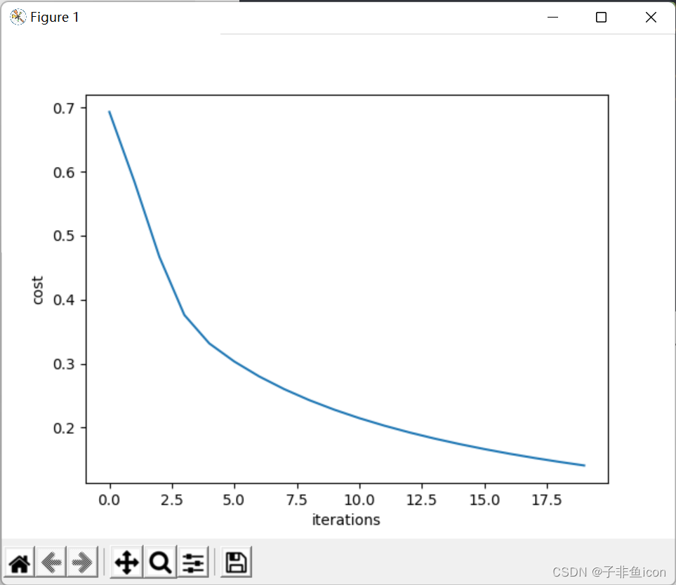
costs = d["cost_ls"]
plt.plot(costs)
plt.xlabel("iterations")
plt.ylabel("cost")
plt.show()
lr_utils.py
import numpy as np
import h5py


def load_dataset():
    train_dataset = h5py.File('datasets/train_catvnoncat.h5', "r")
    train_set_x_orig = np.array(train_dataset["train_set_x"][:]) # your train set features
    train_set_y_orig = np.array(train_dataset["train_set_y"][:]) # your train set labels

    test_dataset = h5py.File('datasets/test_catvnoncat.h5', "r")
    test_set_x_orig = np.array(test_dataset["test_set_x"][:]) # your test set features
    test_set_y_orig = np.array(test_dataset["test_set_y"][:]) # your test set labels

    classes = np.array(test_dataset["list_classes"][:]) # the list of classes

    train_set_y_orig = train_set_y_orig.reshape((1, train_set_y_orig.shape[0]))
    test_set_y_orig = test_set_y_orig.reshape((1, test_set_y_orig.shape[0]))

    return train_set_x_orig, train_set_y_orig, test_set_x_orig, test_set_y_orig, classes
输出结果:

(64, 64, 3)
y=[1], it's a 'cat' picture
(209, 64, 64, 3)
(1, 209)
(50, 64, 64, 3)
(1, 50)
训练集的样本数:209
测试集的样本数:50
图片的宽和高:64
(12288, 209)
(12288, 50)
0 -----> 0.6931471805599453
100 -----> 0.5845083636993086
200 -----> 0.46694904094655465
300 -----> 0.3760068669480207
400 -----> 0.33146328932825125
500 -----> 0.3032730674743828
600 -----> 0.27987958658260487
700 -----> 0.26004213692587563
800 -----> 0.24294068467796612
900 -----> 0.2280042225672607
1000 -----> 0.21481951378449637
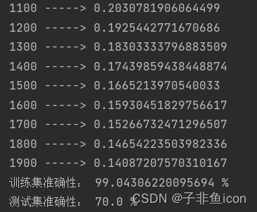
1100 -----> 0.2030781906064499
1200 -----> 0.1925442771670686
1300 -----> 0.18303333796883509
1400 -----> 0.17439859438448874
1500 -----> 0.1665213970540033
1600 -----> 0.15930451829756617
1700 -----> 0.15266732471296507
1800 -----> 0.14654223503982336
1900 -----> 0.14087207570310167
训练集准确性: 99.04306220095694 %
测试集准确性: 70.0 %
{'cost_ls': [0.6931471805599453, 0.5845083636993086, 0.46694904094655465, 0.3760068669480207, 0.33146328932825125, 0.3032730674743828, 0.27987958658260487, 0.26004213692587563, 0.24294068467796612, 0.2280042225672607, 0.21481951378449637, 0.2030781906064499, 0.1925442771670686, 0.18303333796883509, 0.17439859438448874, 0.1665213970540033, 0.15930451829756617, 0.15266732471296507, 0.14654223503982336, 0.14087207570310167], 'y_pred_train': array([[0., 0., 1., 0., 0., 0., 0., 1., 0., 0., 0., 1., 0., 1., 1., 0.,
0., 0., 0., 1., 0., 0., 0., 0., 1., 1., 0., 1., 0., 1., 0., 0.,
0., 0., 0., 0., 0., 0., 1., 0., 0., 0., 1., 0., 0., 0., 0., 1.,
0., 0., 1., 0., 0., 0., 1., 0., 1., 1., 0., 1., 1., 1., 0., 0.,
0., 0., 0., 0., 1., 0., 0., 1., 0., 0., 0., 1., 0., 0., 0., 0.,
0., 0., 0., 1., 1., 0., 0., 0., 1., 0., 0., 0., 1., 1., 1., 0.,
0., 1., 0., 0., 0., 0., 1., 0., 1., 0., 1., 1., 1., 1., 1., 1.,
0., 0., 0., 0., 0., 1., 0., 0., 0., 1., 0., 0., 1., 0., 1., 0.,
1., 1., 0., 0., 0., 1., 1., 1., 1., 1., 0., 0., 0., 0., 1., 0.,
1., 1., 1., 0., 1., 1., 0., 0., 0., 1., 0., 0., 1., 0., 0., 0.,
0., 0., 1., 0., 1., 0., 1., 0., 0., 1., 1., 1., 0., 0., 1., 1.,
0., 1., 0., 1., 0., 0., 0., 0., 0., 1., 0., 0., 1., 0., 0., 0.,
1., 0., 0., 0., 0., 1., 0., 0., 1., 0., 0., 0., 0., 0., 0., 0.,
0.]]), 'y_pred_test': array([[1., 1., 1., 1., 1., 1., 0., 1., 1., 1., 0., 0., 1., 1., 0., 1.,
0., 1., 0., 0., 1., 0., 0., 1., 1., 1., 1., 0., 0., 1., 0., 1.,
1., 0., 1., 0., 0., 1., 0., 0., 1., 0., 1., 0., 1., 0., 0., 1.,
1., 0.]]), 'W': array([[ 0.00961402],
[-0.0264683 ],
[-0.01226513],
...,
[-0.01144453],
[-0.02944783],
[ 0.02378106]]), 'b': -0.01590624399969292}
3.2 将学习率lr设置的比较大的时候,会遇到RuntimeWarning: divide by zero encountered in log警告
是因为sigmoid函数进行exp(-z)运算时,因为输入得z值太大(正值)或太小(负值),产生了内存溢出,最终得到的结果是nan。所以在cost函数中的log计算引发此警告。
比如将lr设置为0.5:
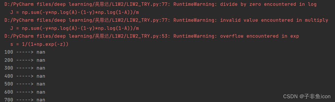
直接报错!
修改为0.005就正常了。
3.3 测试集的准确率始终为34%,而前面的代码经测试均没问题
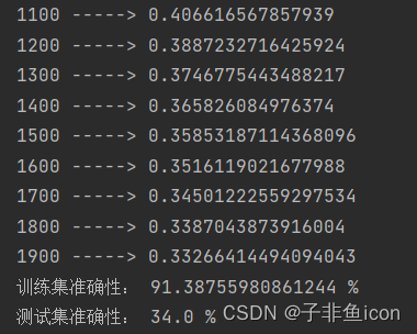
原因如下:
在修改原输入数据时,不能采用注释掉的那一种形式,而应该使用参考链接的,-1放在后面的形式。这是因为:numpy使用reshape时,会先从axis=0填充数据,故用博主的方式可以保证每一行(转置后的每一列)的数据都来自同一图片。而如果train_set_x_orig.shape[0]放在后面,则无法保证来自同一张图片。
下面观察这两种形式,第一列的输入特征(第一张图)有何不同:
第一张图片大概是:
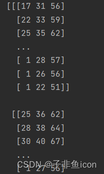
而两者的结果:

从结果来看,只有后者的数据才能保证来自同一图片。
修改后的预测结果:
3.4 尝试增加上面单元格中的迭代次数(修改为3000),可能会看到训练集准确性提高了,但是测试集准确性却降低了。 这称为过度拟合。
3.5 拎出一张图片查看预测结果
测试集第11张
# 图片对比查看
index_t = 10
plt.imshow(test_set_x[:,index_t].reshape((num_px, num_px, 3)))
plt.show()

print("y=" + str(test_set_y[:,index_t]) + ", You predicted that it is a '" + classes[int(d["y_pred_test"][:, index_t])].decode("utf-8") + "' picture")
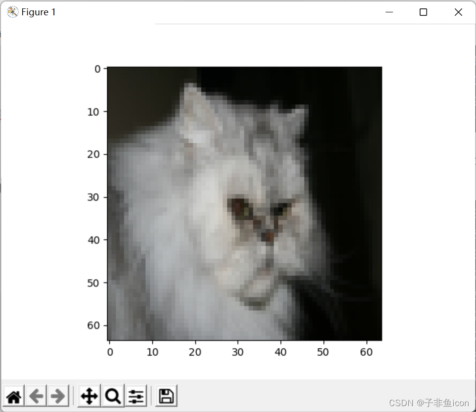
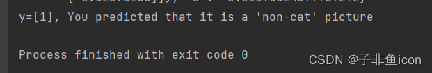
然后就发现它预测错了。。。
3.6 超参数——学习率的选择
学习率决定我们更新参数的速度。 如果学习率太大,我们可能会“超出”最佳值。 同样,如果太小,将需要更多的迭代才能收敛到最佳值。
# 学习率的选择
learning_rates = [0.01, 0.001, 0.0001]
models = {}
for i in learning_rates:
    print ("learning rate is: " + str(i))
    models[str(i)] = model(train_set_x, train_set_y, test_set_x, test_set_y, num_iterations = 1500, lr = i, show_cost = False)
    print ('\n' + "-------------------------------------------------------" + '\n')

for i in learning_rates:
    plt.plot(np.squeeze(models[str(i)]["cost_ls"]), label= str(models[str(i)]["lr"]))

plt.ylabel('cost')
plt.xlabel('iterations')

legend = plt.legend(loc='upper center', shadow=True)
frame = legend.get_frame()   # 获得背景
frame.set_facecolor('0.90') # 设置背景透明度
plt.show()
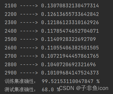
结果:
learning rate is: 0.01
训练集准确性: 99.52153110047847 %
测试集准确性: 68.0 %

-------------------------------------------------------

learning rate is: 0.001
训练集准确性: 88.99521531100478 %
测试集准确性: 64.0 %

-------------------------------------------------------

learning rate is: 0.0001
训练集准确性: 68.42105263157895 %
测试集准确性: 36.0 %

-------------------------------------------------------


Process finished with exit code 0
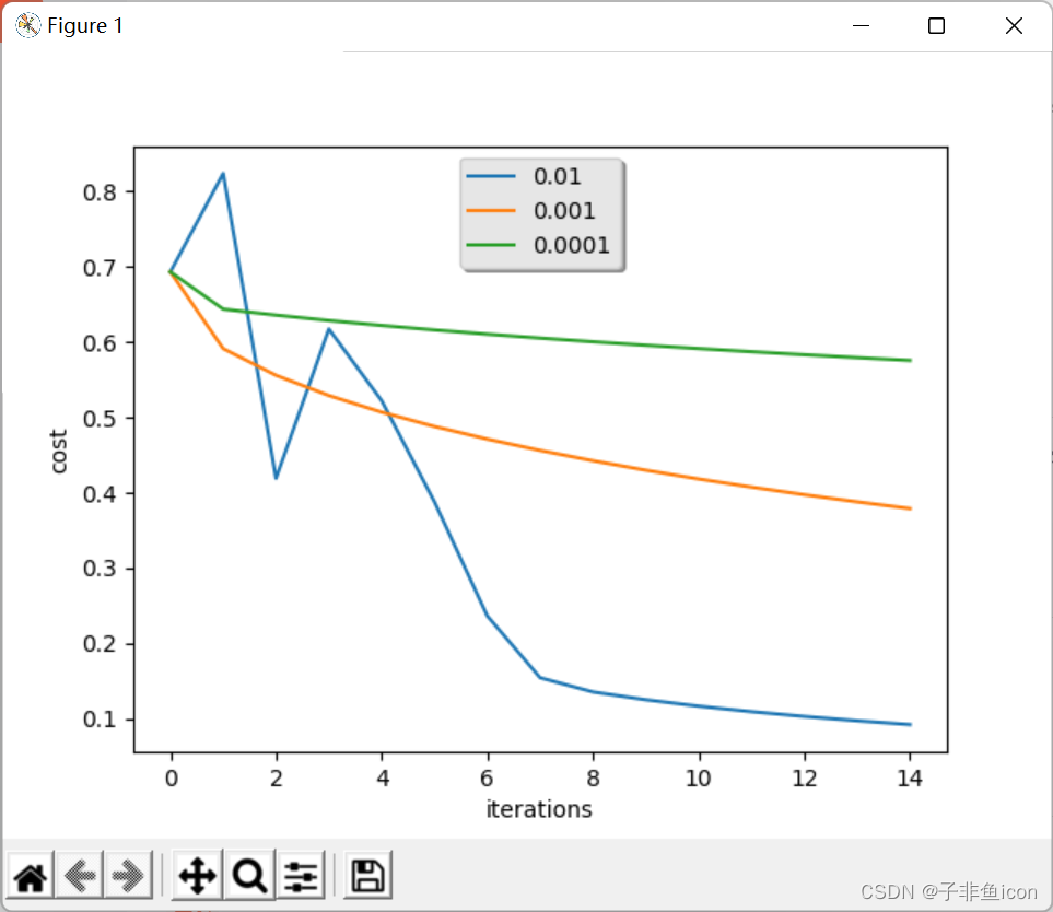
不同的学习率会带来不同的损失,因此会有不同的预测结果。
如果学习率太大(0.01),则成本可能会上下波动。 它甚至可能会发散(尽管在此示例中,使用0.01最终仍会以较高的损失值获得收益)。
较低的损失并不意味着模型效果很好。当训练精度比测试精度高很多时,就会发生过拟合情况。
在深度学习中,通常建议:
1.选择好能最小化损失函数的学习率。
2.如果模型过度拟合,请使用其他方法来减少过度拟合。
3.7 使用其他的猫猫图
网上下载的:

程序:
# 使用其他的猫猫图
fname = "D:\PyCharm files\deep learning\吴恩达\L1W2\cat.jpeg"
image = np.array(plt.imread(fname))
print(image.shape)

from skimage.transform import resize

my_image = resize(image,output_shape=(num_px,num_px))  # 修改尺寸为64*64
plt.imshow(my_image)
plt.show()

my_image = my_image.reshape((1, num_px*num_px*3)).T  # 转换成向量便于预测
print(my_image.shape)
#my_image = scipy.misc.imresize(image, size=(num_px,num_px)).reshape((1, num_px*num_px*3)).T
my_predicted_image = predict(d["W"], d["b"], my_image)
print("y = " + str(np.squeeze(my_predicted_image)) + ", your algorithm predicts a \"" + classes[int(np.squeeze(my_predicted_image)),].decode("utf-8") +  "\" picture.")
此处按照参考链接的可能会报错,是因为scipy的版本问题。参考链接
经过程序修改尺寸为64×64后
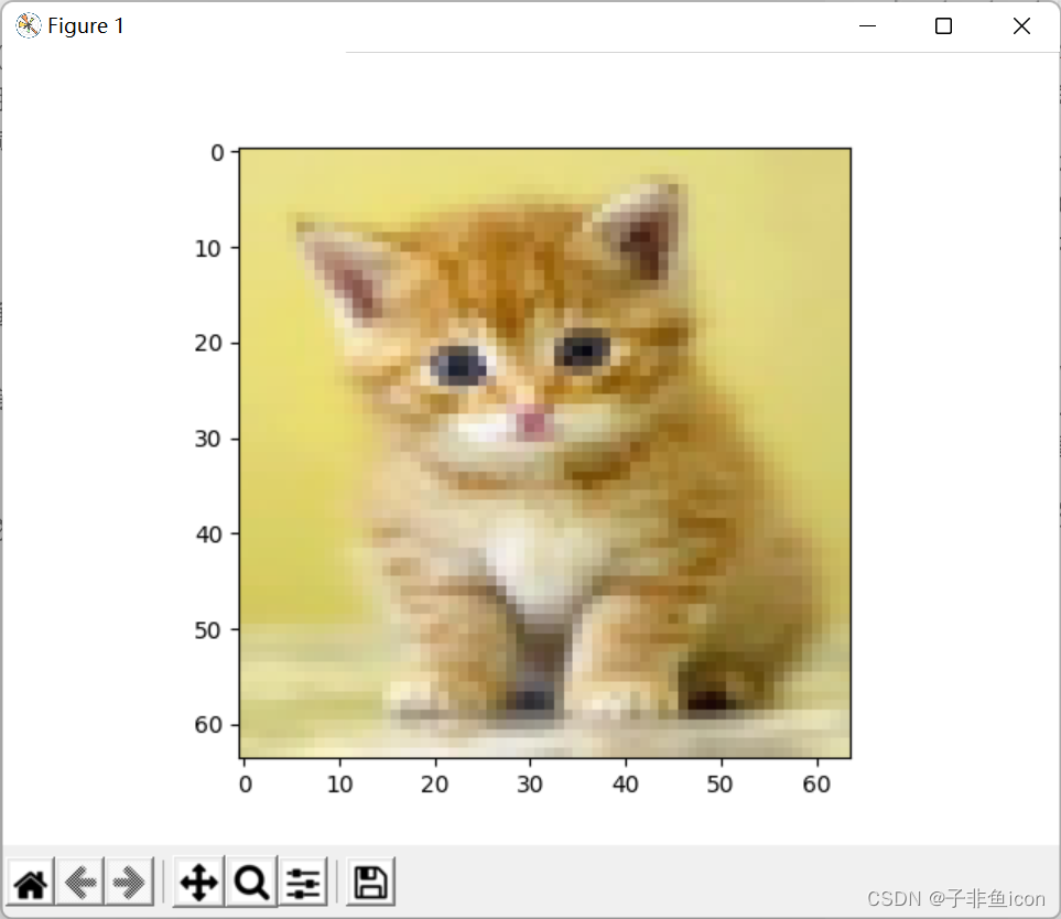
输出:
(220, 176, 3)
(12288, 1)
[[0.]]
y = 0.0, your algorithm predicts a "non-cat" picture.
嗯…识别失败,证明这个神经网络模型,的确有待提高。


 89
89


 被折叠的 条评论
为什么被折叠?
被折叠的 条评论
为什么被折叠?
 到【灌水乐园】发言


