


文章目录
一、使用PyTorch实现反向传播和梯度下降
1.使用PyTorch实现模型
激活函数使用Sigmoid函数
损失函数使用均方误差MSE
使用PyTorch新建权重向量并确定是否需要求梯度
w1, w2, w3, w4, w5, w6, w7, w8 = torch.Tensor([0.2]), torch.Tensor([-0.4]), torch.Tensor([0.5]), torch.Tensor(
    [0.6]), torch.Tensor([0.1]), torch.Tensor([-0.5]), torch.Tensor([-0.3]), torch.Tensor([0.8])  # 权重初始值
w1.requires_grad = True
w2.requires_grad = True
w3.requires_grad = True
w4.requires_grad = True
w5.requires_grad = True
w6.requires_grad = True
w7.requires_grad = True
w8.requires_grad = True
将前向传播过程转化为各个计算表达式,最终表示出损失函数
    in_h1 = w1 * x1 + w3 * x2
    out_h1 = sigmoid(in_h1)  # out_h1 = torch.sigmoid(in_h1)
    in_h2 = w2 * x1 + w4 * x2
    out_h2 = sigmoid(in_h2)  # out_h2 = torch.sigmoid(in_h2)

    in_o1 = w5 * out_h1 + w7 * out_h2
    out_o1 = sigmoid(in_o1)  # out_o1 = torch.sigmoid(in_o1)
    in_o2 = w6 * out_h1 + w8 * out_h2
    out_o2 = sigmoid(in_o2)  # out_o2 = torch.sigmoid(in_o2)
	def loss_fuction(x1, x2, y1, y2):  # 损失函数
    y1_pred, y2_pred = forward_propagate(x1, x2)  # 前向传播
    loss = (1 / 2) * (y1_pred - y1) ** 2 + (1 / 2) * (y2_pred - y2) ** 2  # 考虑 : t.nn.MSELoss()
    print("损失函数(均方误差):", loss.item())
    return loss
对损失函数调用PyTorch反向传播,计算出梯度
L.backward()
更新梯度下降更新权重向量
    step = 1
    w1.data = w1.data - step * w1.grad.data
    w2.data = w2.data - step * w2.grad.data
    w3.data = w3.data - step * w3.grad.data
    w4.data = w4.data - step * w4.grad.data
    w5.data = w5.data - step * w5.grad.data
    w6.data = w6.data - step * w6.grad.data
    w7.data = w7.data - step * w7.grad.data
    w8.data = w8.data - step * w8.grad.data
    w1.grad.data.zero_()  # 注意:将w中所有梯度清零
    w2.grad.data.zero_()
    w3.grad.data.zero_()
    w4.grad.data.zero_()
    w5.grad.data.zero_()
    w6.grad.data.zero_()
    w7.grad.data.zero_()
    w8.grad.data.zero_()
    return w1, w2, w3, w4, w5, w6, w7, w8
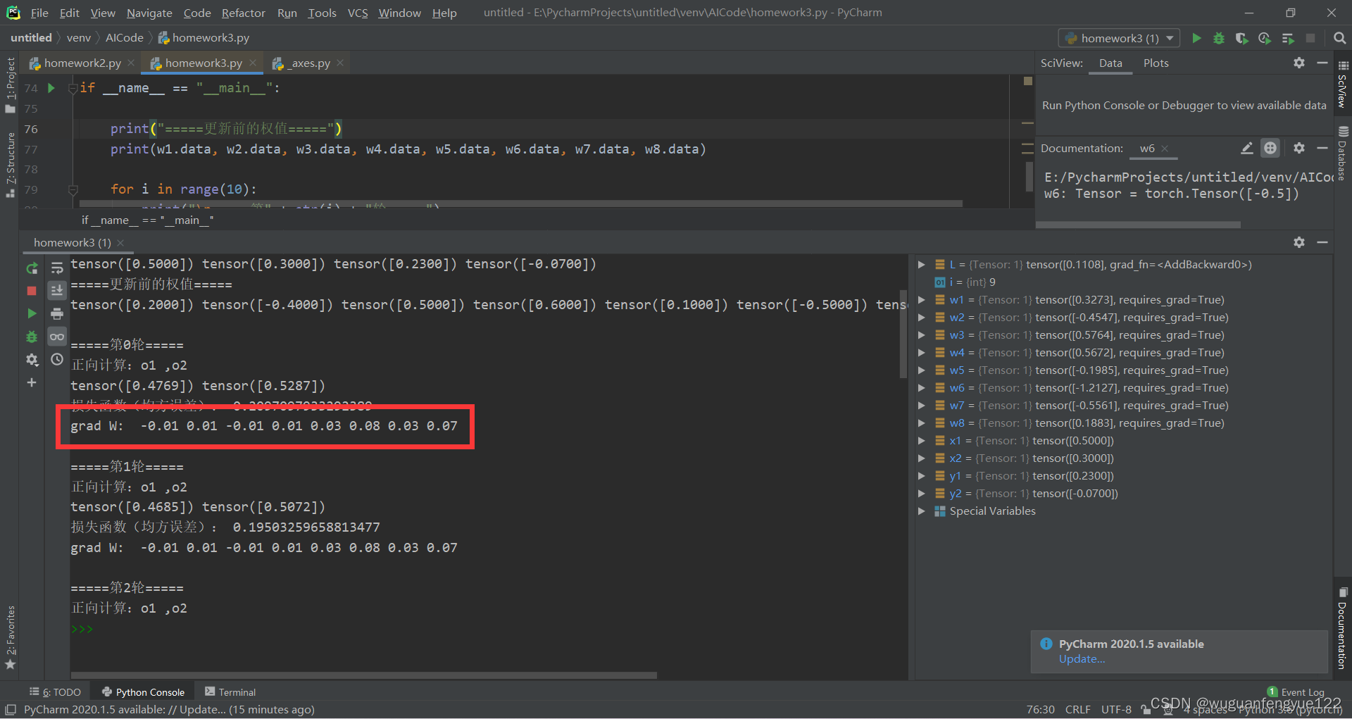
将反向传播,提取下降的过程重复多次,观察算法的收敛性
    for i in range(10):
        print("\n=====第" + str(i) + "轮=====")
        L = loss_fuction(x1, x2, y1, y2)  # 前向传播,求 Loss,构建计算图
        L.backward()  # 自动求梯度,不需要人工编程实现。反向传播,求出计算图中所有梯度存入w中
        print("grad W: ", round(w1.grad.item(), 2), round(w2.grad.item(), 2), round(w3.grad.item(), 2),
              round(w4.grad.item(), 2), round(w5.grad.item(), 2), round(w6.grad.item(), 2), round(w7.grad.item(), 2),
              round(w8.grad.item(), 2))
        w1, w2, w3, w4, w5, w6, w7, w8 = update_w(w1, w2, w3, w4, w5, w6, w7, w8)

    print("更新后的权值")
    print(w1.data, w2.data, w3.data, w4.data, w5.data, w6.data, w7.data, w8.data)
完整代码
# https://blog.csdn.net/qq_41033011/article/details/109325070
# https://github.com/Darwlr/Deep_learning/blob/master/06%20Pytorch%E5%AE%9E%E7%8E%B0%E5%8F%8D%E5%90%91%E4%BC%A0%E6%92%AD.ipynb
# torch.nn.Sigmoid(h_in)

import torch

x1, x2 = torch.Tensor([0.5]), torch.Tensor([0.3])
y1, y2 = torch.Tensor([0.23]), torch.Tensor([-0.07])
print("=====输入值:x1, x2;真实输出值:y1, y2=====")
print(x1, x2, y1, y2)
w1, w2, w3, w4, w5, w6, w7, w8 = torch.Tensor([0.2]), torch.Tensor([-0.4]), torch.Tensor([0.5]), torch.Tensor(
    [0.6]), torch.Tensor([0.1]), torch.Tensor([-0.5]), torch.Tensor([-0.3]), torch.Tensor([0.8])  # 权重初始值
w1.requires_grad = True
w2.requires_grad = True
w3.requires_grad = True
w4.requires_grad = True
w5.requires_grad = True
w6.requires_grad = True
w7.requires_grad = True
w8.requires_grad = True


def sigmoid(z):
    a = 1 / (1 + torch.exp(-z))
    return a


def forward_propagate(x1, x2):
    in_h1 = w1 * x1 + w3 * x2
    out_h1 = sigmoid(in_h1)  # out_h1 = torch.sigmoid(in_h1)
    in_h2 = w2 * x1 + w4 * x2
    out_h2 = sigmoid(in_h2)  # out_h2 = torch.sigmoid(in_h2)

    in_o1 = w5 * out_h1 + w7 * out_h2
    out_o1 = sigmoid(in_o1)  # out_o1 = torch.sigmoid(in_o1)
    in_o2 = w6 * out_h1 + w8 * out_h2
    out_o2 = sigmoid(in_o2)  # out_o2 = torch.sigmoid(in_o2)

    print("正向计算:o1 ,o2")
    print(out_o1.data, out_o2.data)

    return out_o1, out_o2


def loss_fuction(x1, x2, y1, y2):  # 损失函数
    y1_pred, y2_pred = forward_propagate(x1, x2)  # 前向传播
    loss = (1 / 2) * (y1_pred - y1) ** 2 + (1 / 2) * (y2_pred - y2) ** 2  # 考虑 : t.nn.MSELoss()
    print("损失函数(均方误差):", loss.item())
    return loss


def update_w(w1, w2, w3, w4, w5, w6, w7, w8):
    # 步长
    step = 1
    w1.data = w1.data - step * w1.grad.data
    w2.data = w2.data - step * w2.grad.data
    w3.data = w3.data - step * w3.grad.data
    w4.data = w4.data - step * w4.grad.data
    w5.data = w5.data - step * w5.grad.data
    w6.data = w6.data - step * w6.grad.data
    w7.data = w7.data - step * w7.grad.data
    w8.data = w8.data - step * w8.grad.data
    w1.grad.data.zero_()  # 注意:将w中所有梯度清零
    w2.grad.data.zero_()
    w3.grad.data.zero_()
    w4.grad.data.zero_()
    w5.grad.data.zero_()
    w6.grad.data.zero_()
    w7.grad.data.zero_()
    w8.grad.data.zero_()
    return w1, w2, w3, w4, w5, w6, w7, w8


if __name__ == "__main__":

    print("=====更新前的权值=====")
    print(w1.data, w2.data, w3.data, w4.data, w5.data, w6.data, w7.data, w8.data)

    for i in range(10):
        print("\n=====第" + str(i) + "轮=====")
        L = loss_fuction(x1, x2, y1, y2)  # 前向传播,求 Loss,构建计算图
        L.backward()  # 自动求梯度,不需要人工编程实现。反向传播,求出计算图中所有梯度存入w中
        print("grad W: ", round(w1.grad.item(), 2), round(w2.grad.item(), 2), round(w3.grad.item(), 2),
              round(w4.grad.item(), 2), round(w5.grad.item(), 2), round(w6.grad.item(), 2), round(w7.grad.item(), 2),
              round(w8.grad.item(), 2))
        w1, w2, w3, w4, w5, w6, w7, w8 = update_w(w1, w2, w3, w4, w5, w6, w7, w8)

    print("更新后的权值")
    print(w1.data, w2.data, w3.data, w4.data, w5.data, w6.data, w7.data, w8.data)
2.对比手动实现反向传播和使用PyTorch的结果
PyTorch第一轮反向传播求得的梯度
手动计算第一轮反向传播求得的梯度
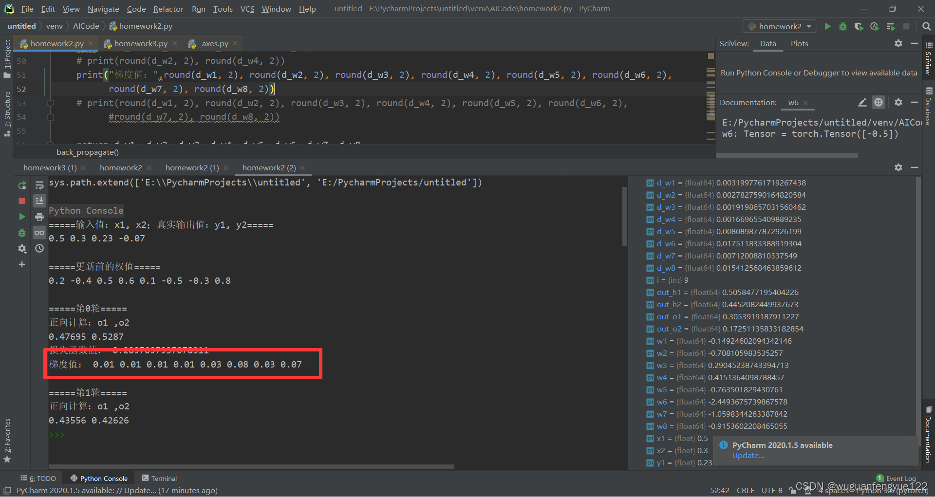
可以发现第一轮反向传播中,手动计算和使用PyTorch计算的权重向量的梯度值只有w1和w3互为相反数,其他相同。
3.手动计算和使用PyTorch求梯度的比较和总结
很明显作为一个成熟的机器学习库,PyTorch能够简化极大的简化神经网络模型中的反向传播求各个参数的梯度问题,其实在明确了模型和损失函数之后,使用PyTorch反向传播求梯度只需要使用loss.backward就可求得权重向量的梯度。
手动计算可以可以作为初学者在计算简单模型时理解反向传播的原理时与PyTorch结果对照比较,并不适用在实际应用中,尤其当实际模型的隐藏层高达几十层甚至数百层,手动计算不仅效率的而且容易出错。
二、更改激活函数
1.激活函数改用PyTorch自带函数torch.sigmoid()
在前向传播计算损失函数的过程中将定义的sigmoid函数换成PyTorch的sigmoid函数
原函数:
def sigmoid(z):
    a = 1 / (1 + torch.exp(-z))
    return a


def forward_propagate(x1, x2):
    in_h1 = w1 * x1 + w3 * x2
    out_h1 = sigmoid(in_h1)
    in_h2 = w2 * x1 + w4 * x2
    out_h2 = sigmoid(in_h2)

    in_o1 = w5 * out_h1 + w7 * out_h2
    out_o1 = sigmoid(in_o1)
    in_o2 = w6 * out_h1 + w8 * out_h2
    out_o2 = sigmoid(in_o2)

    print("正向计算:o1 ,o2")
    print(out_o1.data, out_o2.data)

    return out_o1, out_o2
替换后的函数:
def forward_propagate(x1, x2):
    in_h1 = w1 * x1 + w3 * x2
    out_h1 = torch.sigmoid(in_h1)
    in_h2 = w2 * x1 + w4 * x2
    out_h2 = torch.sigmoid(in_h2)

    in_o1 = w5 * out_h1 + w7 * out_h2
    out_o1 = torch.sigmoid(in_o1)
    in_o2 = w6 * out_h1 + w8 * out_h2
    out_o2 = torch.sigmoid(in_o2)

    print("正向计算:o1 ,o2")
    print(out_o1.data, out_o2.data)

    return out_o1, out_o2
程序运行的结果:
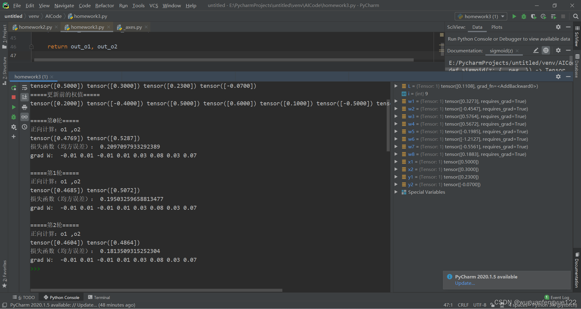
=====输入值:x1, x2;真实输出值:y1, y2=====
tensor([0.5000]) tensor([0.3000]) tensor([0.2300]) tensor([-0.0700])
=====更新前的权值=====
tensor([0.2000]) tensor([-0.4000]) tensor([0.5000]) tensor([0.6000]) tensor([0.1000]) tensor([-0.5000]) tensor([-0.3000]) tensor([0.8000])
=====第0轮=====
正向计算:o1 ,o2
tensor([0.4769]) tensor([0.5287])
损失函数(均方误差): 0.2097097933292389
grad W:  -0.01 0.01 -0.01 0.01 0.03 0.08 0.03 0.07
=====第1轮=====
正向计算:o1 ,o2
tensor([0.4685]) tensor([0.5072])
损失函数(均方误差): 0.19503259658813477
grad W:  -0.01 0.01 -0.01 0.01 0.03 0.08 0.03 0.07
=====第2轮=====
正向计算:o1 ,o2
tensor([0.4604]) tensor([0.4864])
损失函数(均方误差): 0.1813509315252304
grad W:  -0.01 0.01 -0.01 0.01 0.03 0.08 0.03 0.07
=====第3轮=====
正向计算:o1 ,o2
tensor([0.4526]) tensor([0.4664])
损失函数(均方误差): 0.16865134239196777
grad W:  -0.01 0.01 -0.01 0.0 0.03 0.08 0.03 0.07
=====第4轮=====
正向计算:o1 ,o2
tensor([0.4451]) tensor([0.4473])
损失函数(均方误差): 0.15690487623214722
grad W:  -0.01 0.01 -0.01 0.0 0.03 0.07 0.03 0.06
=====第5轮=====
正向计算:o1 ,o2
tensor([0.4378]) tensor([0.4290])
损失函数(均方误差): 0.14607082307338715
grad W:  -0.01 0.0 -0.01 0.0 0.03 0.07 0.02 0.06
=====第6轮=====
正向计算:o1 ,o2
tensor([0.4307]) tensor([0.4116])
损失函数(均方误差): 0.1361003816127777
grad W:  -0.01 0.0 -0.01 0.0 0.03 0.07 0.02 0.06
=====第7轮=====
正向计算:o1 ,o2
tensor([0.4239]) tensor([0.3951])
损失函数(均方误差): 0.1269397884607315
grad W:  -0.01 0.0 -0.01 0.0 0.03 0.06 0.02 0.05
=====第8轮=====
正向计算:o1 ,o2
tensor([0.4173]) tensor([0.3794])
损失函数(均方误差): 0.11853284388780594
grad W:  -0.01 0.0 -0.01 0.0 0.03 0.06 0.02 0.05
=====第9轮=====
正向计算:o1 ,o2
tensor([0.4109]) tensor([0.3647])
损失函数(均方误差): 0.11082295328378677
grad W:  -0.02 0.0 -0.01 0.0 0.03 0.06 0.02 0.05
更新后的权值
tensor([0.3273]) tensor([-0.4547]) tensor([0.5764]) tensor([0.5672]) tensor([-0.1985]) tensor([-1.2127]) tensor([-0.5561]) tensor([0.1883])
2.激活函数Sigmoid改变为Relu
将损失函数换为Relu
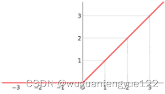
Relu函数的表达式为:f(x) = max(0,x)
图像如下:
原函数:
def forward_propagate(x1, x2):
    in_h1 = w1 * x1 + w3 * x2
    out_h1 = torch.sigmoid(in_h1)
    in_h2 = w2 * x1 + w4 * x2
    out_h2 = torch.sigmoid(in_h2)

    in_o1 = w5 * out_h1 + w7 * out_h2
    out_o1 = torch.sigmoid(in_o1)
    in_o2 = w6 * out_h1 + w8 * out_h2
    out_o2 = torch.sigmoid(in_o2)

    print("正向计算:o1 ,o2")
    print(out_o1.data, out_o2.data)

    return out_o1, out_o2
更换后的函数:
def forward_propagate(x1, x2):
    in_h1 = w1 * x1 + w3 * x2
    out_h1 = torch.relu(in_h1)
    in_h2 = w2 * x1 + w4 * x2
    out_h2 = torch.relu(in_h2)


    in_o1 = w5 * out_h1 + w7 * out_h2
    out_o1 = torch.relu(in_o1)
    in_o2 = w6 * out_h1 + w8 * out_h2
    out_o2 = torch.relu(in_o2)

    print("正向计算:o1 ,o2")
    print(out_o1.data, out_o2.data)

    return out_o1, out_o2
程序运行的结果:
=====输入值:x1, x2;真实输出值:y1, y2=====
tensor([0.5000]) tensor([0.3000]) tensor([0.2300]) tensor([-0.0700])
=====更新前的权值=====
tensor([0.2000]) tensor([-0.4000]) tensor([0.5000]) tensor([0.6000]) tensor([0.1000]) tensor([-0.5000]) tensor([-0.3000]) tensor([0.8000])
=====第0轮=====
正向计算:o1 ,o2
tensor([0.0250]) tensor([0.])
损失函数(均方误差): 0.023462500423192978
grad W:  -0.01 0.0 -0.01 0.0 -0.05 0.0 -0.0 0.0
=====第1轮=====
正向计算:o1 ,o2
tensor([0.0389]) tensor([0.])
损失函数(均方误差): 0.020715968683362007
grad W:  -0.01 0.0 -0.01 0.0 -0.05 0.0 0.0 0.0
=====第2轮=====
正向计算:o1 ,o2
tensor([0.0535]) tensor([0.])
损失函数(均方误差): 0.01803365722298622
grad W:  -0.02 0.0 -0.01 0.0 -0.05 0.0 0.0 0.0
=====第3轮=====
正向计算:o1 ,o2
tensor([0.0690]) tensor([0.])
损失函数(均方误差): 0.015410471707582474
grad W:  -0.02 0.0 -0.01 0.0 -0.04 0.0 0.0 0.0
=====第4轮=====
正向计算:o1 ,o2
tensor([0.0855]) tensor([0.])
损失函数(均方误差): 0.012893404811620712
grad W:  -0.02 0.0 -0.01 0.0 -0.04 0.0 0.0 0.0

=====第5轮=====
正向计算:o1 ,o2
tensor([0.1026]) tensor([0.])
损失函数(均方误差): 0.010560503229498863
grad W:  -0.02 0.0 -0.01 0.0 -0.04 0.0 0.0 0.0
=====第6轮=====
正向计算:o1 ,o2
tensor([0.1200]) tensor([0.])
损失函数(均方误差): 0.008496038615703583
grad W:  -0.02 0.0 -0.01 0.0 -0.04 0.0 0.0 0.0
=====第7轮=====
正向计算:o1 ,o2
tensor([0.1371]) tensor([0.])
损失函数(均方误差): 0.006765476893633604
grad W:  -0.02 0.0 -0.01 0.0 -0.03 0.0 0.0 0.0
=====第8轮=====
正向计算:o1 ,o2
tensor([0.1532]) tensor([0.])
损失函数(均方误差): 0.005397447384893894
grad W:  -0.02 0.0 -0.01 0.0 -0.03 0.0 0.0 0.0
=====第9轮=====
正向计算:o1 ,o2
tensor([0.1679]) tensor([0.])
损失函数(均方误差): 0.004378797020763159
grad W:  -0.01 0.0 -0.01 0.0 -0.02 0.0 0.0 0.0
更新后的权值
tensor([0.3757]) tensor([-0.4000]) tensor([0.6054]) tensor([0.6000]) tensor([0.4892]) tensor([-0.5000]) tensor([-0.3000]) tensor([0.8000])
三、更换损失函数
1.使用PyTorch计算损失函数
修改计算损失函数代码为:
def loss_fuction(x1, x2, y1, y2):  # 损失函数
    # torch.nn.CrossEntropyLoss交叉熵
    y1_pred, y2_pred = forward_propagate(x1, x2)  # 前向传播
    loss_f = torch.nn.MSELoss()
    # loss_f = torch.nn.CrossEntropyLoss交叉熵
    y_pred = torch.cat((y1_pred, y2_pred), dim=0)
    y = torch.cat((y1, y2), dim=0)
    loss = loss_f(y_pred,y)
    print("损失函数(均方误差):", loss.item())
    return loss
在计算之前要将所有预测值合并成一个张量,所有实际值合并成一个张量,再使用torch.nn.MSELoss()计算结果
2.使用交叉熵计算损失函数
修改计算损失函数代码为:
def loss_fuction(x1, x2, y1, y2):  # 损失函数
    # torch.nn.CrossEntropyLoss交叉熵
    y1_pred, y2_pred = forward_propagate(x1, x2)  # 前向传播
    # loss_f = torch.nn.MSELoss()
    loss_f = torch.nn.CrossEntropyLoss
    y_pred = torch.cat((y1_pred, y2_pred), dim=0)
    y = torch.cat((y1, y2), dim=0)
    loss = loss_f(y_pred,y)
    print("损失函数(均方误差):", loss.item())
    return loss
四、改变步长
在梯度下降的函数中修改步长观察模型的收敛情况,迭代50轮
def update_w(w1, w2, w3, w4, w5, w6, w7, w8):
    step = 1 #步长,令step = 1,10,50,100
    w1.data = w1.data - step * w1.grad.data
    w2.data = w2.data - step * w2.grad.data
    w3.data = w3.data - step * w3.grad.data
    w4.data = w4.data - step * w4.grad.data
    w5.data = w5.data - step * w5.grad.data
    w6.data = w6.data - step * w6.grad.data
    w7.data = w7.data - step * w7.grad.data
    w8.data = w8.data - step * w8.grad.data
    w1.grad.data.zero_()  # 注意:将w中所有梯度清零
    w2.grad.data.zero_()
    w3.grad.data.zero_()
    w4.grad.data.zero_()
    w5.grad.data.zero_()
    w6.grad.data.zero_()
    w7.grad.data.zero_()
    w8.grad.data.zero_()
    return w1, w2, w3, w4, w5, w6, w7, w8
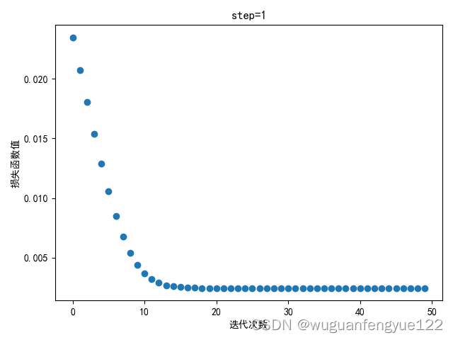
step = 1
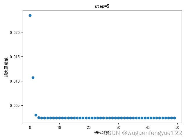
step = 5
step = 10
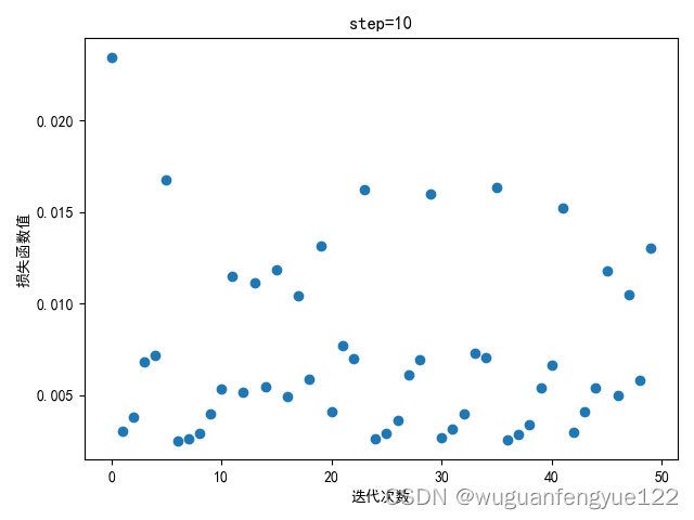
可以观察到当步长到10时梯度下降开始震荡,说明步长过大,模型无法较好的收敛。
五、将初始权重向量赋随机值
使用随机生成的初始步长
# w1, w2, w3, w4, w5, w6, w7, w8 = torch.Tensor([0.2]), torch.Tensor([-0.4]), torch.Tensor([0.5]), torch.Tensor(
#     [0.6]), torch.Tensor([0.1]), torch.Tensor([-0.5]), torch.Tensor([-0.3]), torch.Tensor([0.8])
w1, w2, w3, w4, w5, w6, w7, w8 = torch.randn(1), torch.randn(1), torch.randn(1), torch.randn(1), \
    torch.randn(1), torch.randn(1), torch.randn(1), torch.randn(1)
生成的随机权重值:
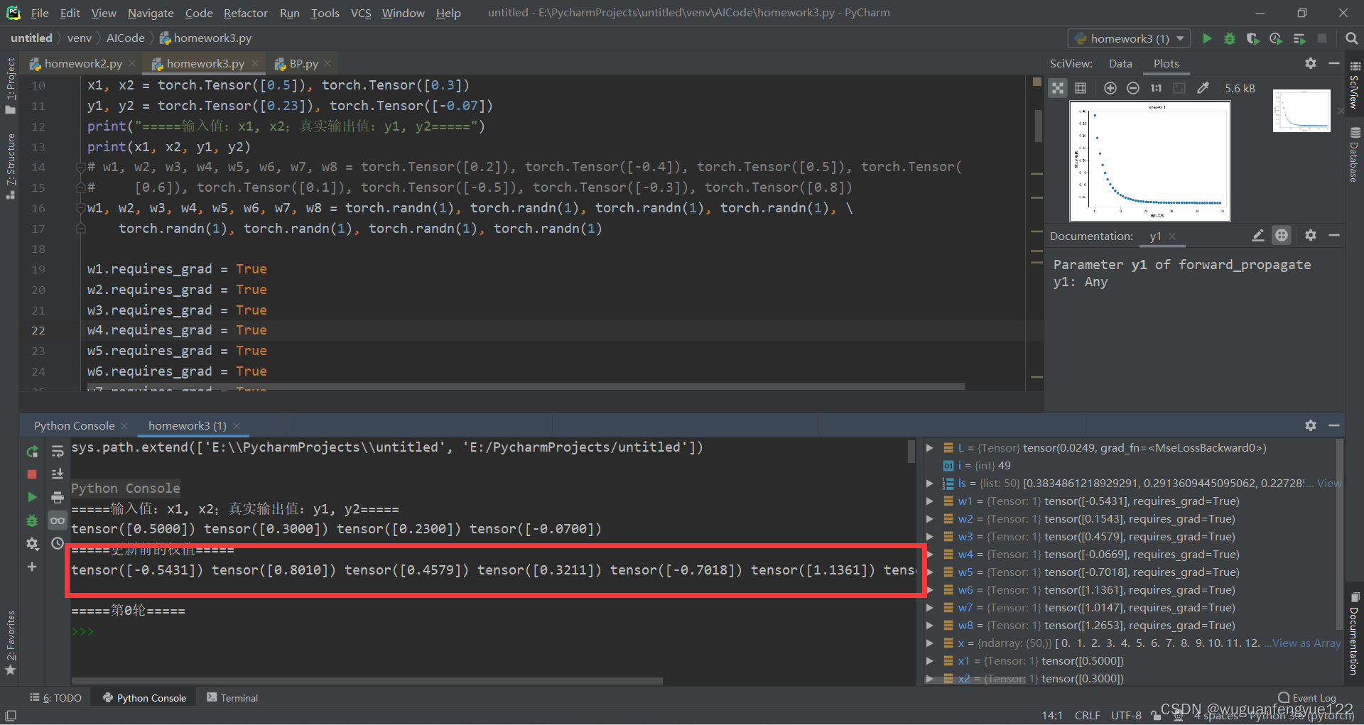
tensor([-0.5431]) tensor([0.8010]) tensor([0.4579]) tensor([0.3211]) tensor([-0.7018]) tensor([1.1361]) tensor([1.0089]) tensor([1.5352])
模型收敛情况(step = 0.1)
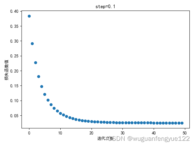
可以观察到模型依旧能较好地收敛。
六、总结
1.神经网络模型
神经网络模型可以分为三层:输入层、隐藏层、输出层。由输入层获得输入数据,经过在层与层之间的前向传播之后最终获得输出损失函数。不同的神经网络模型一般隐藏层层数和结点连接方式不同,也即是层与层之间的传递计算关系不同。
2.反向传播
反向传播是为了梯度下降做准备,实现方法就是计算损失函数对传播路径上每一个权重的偏导数,可以使用PyTorch实现来提高编码效率的准确性。
3.梯度下降
梯度下降就是在计算出损失函数对权重的偏导数:梯度后,沿着损失函数下降最快的方向更新权重值以降低损失函数值,从而提升模型的准确率。
3.PyTorch的使用
使用PyTorch完成反向传播过程中各个权重的梯度计算即快有准确,而且PyTorch还包含了多种封装好的损失函数计算函数,是神经网络模型中十分好用的工具库。


 216
216


 被折叠的 条评论
为什么被折叠?
被折叠的 条评论
为什么被折叠?
 到【灌水乐园】发言


