


👨🎓个人主页:研学社的博客
💥💥💞💞欢迎来到本博客❤️❤️💥💥
🏆博主优势:🌞🌞🌞博客内容尽量做到思维缜密,逻辑清晰,为了方便读者。
⛳️座右铭:行百里者,半于九十。
📋📋📋本文目录如下:🎁🎁🎁
目录

💥1 概述
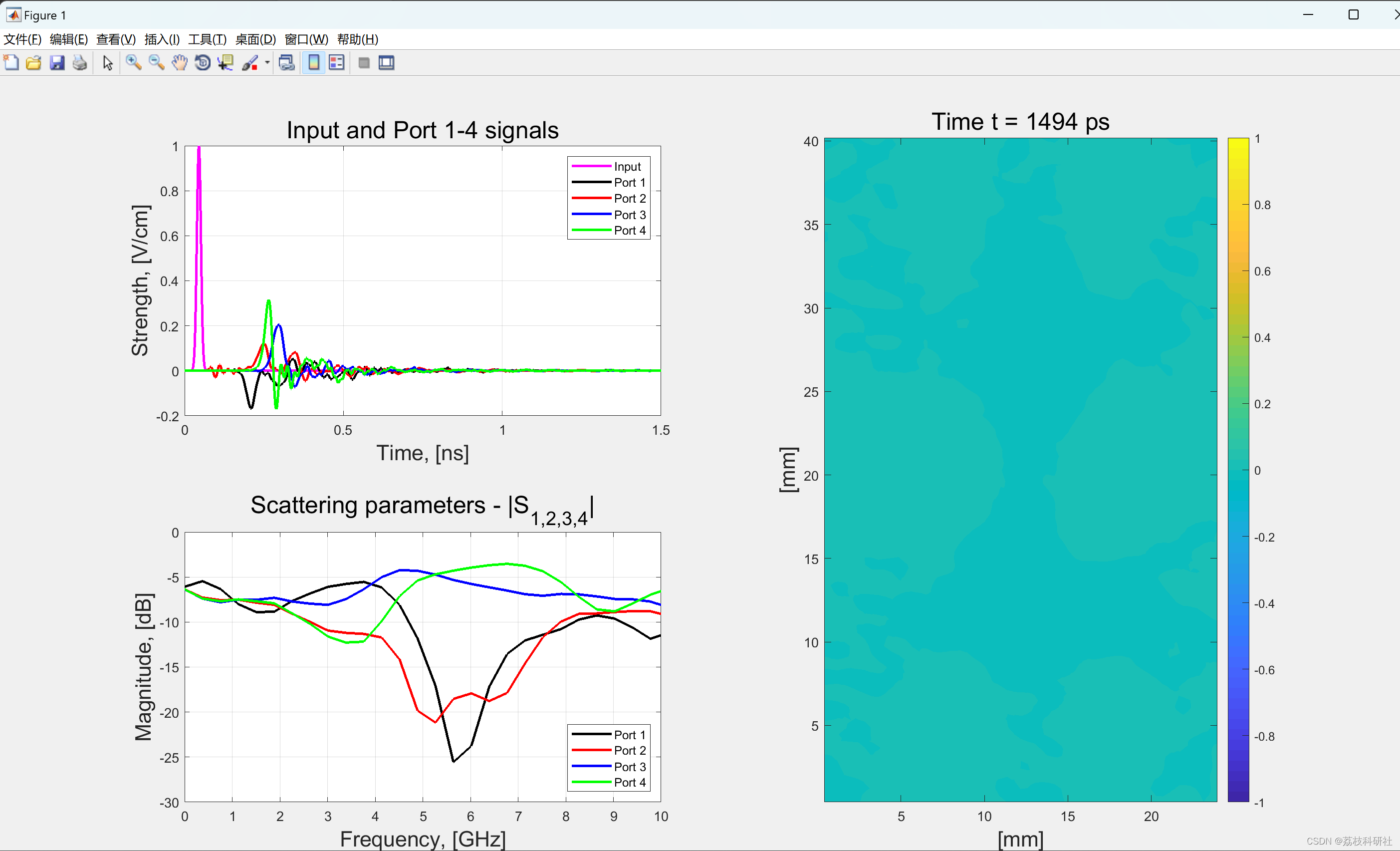
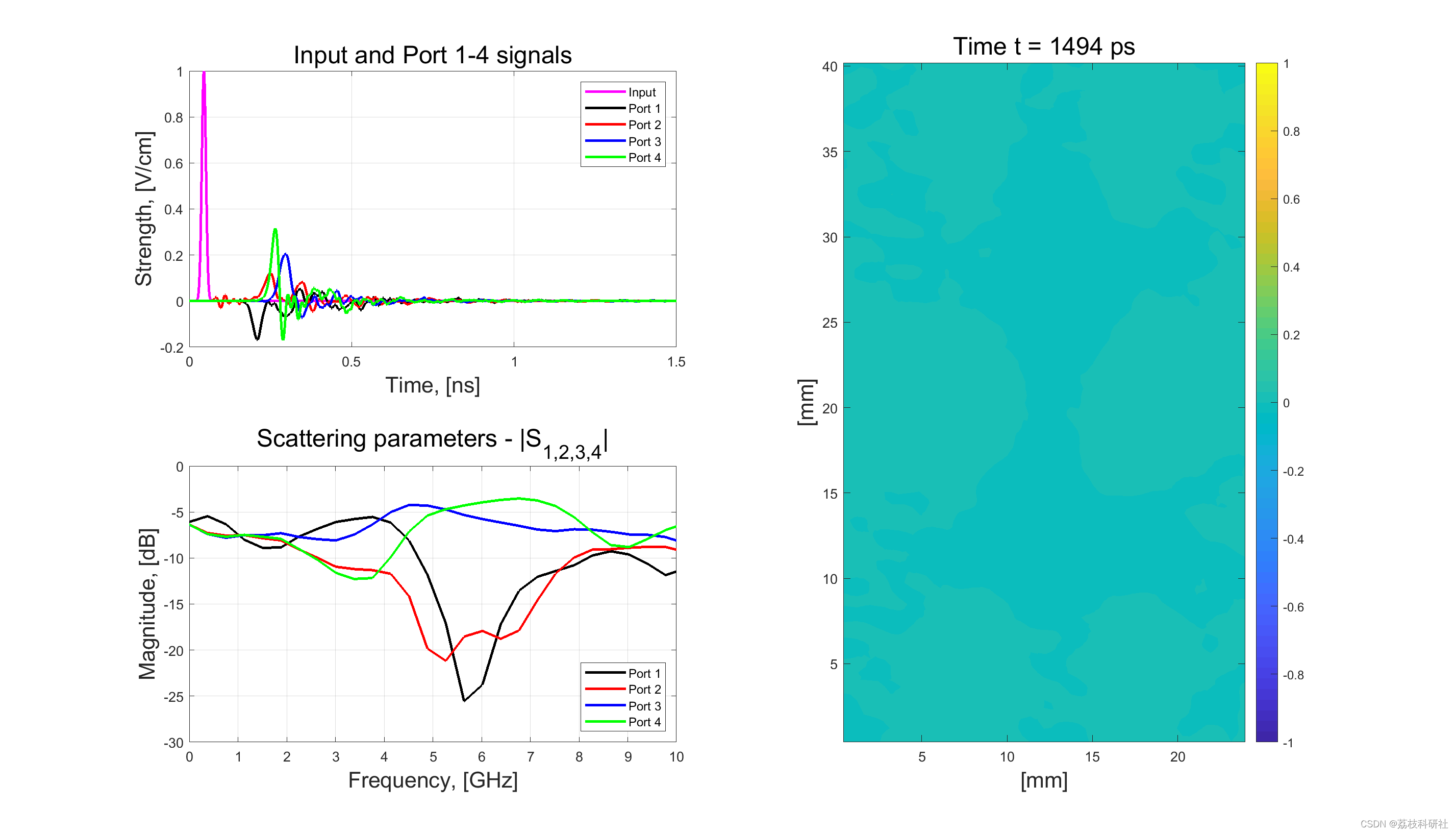
将直接三维有限差分时域(FDTD)方法应用于各种微带结构的全波分析。该方法被证明是模拟复杂微带电路元件和微带天线的有效工具。根据时域结果计算了线馈矩形贴片天线的输入阻抗以及低通滤波器和支线耦合器的频率相关散射参数。这些电路是捏造的,对它们的测量结果与FDTD结果进行了比较,并显示出良好的一致性。
原文摘要:
Abstract:
A direct three-dimensional finite-difference time-domain (FDTD) method is applied to the full-wave analysis of various microstrip structures. The method is shown to be an efficient tool for modeling complicated microstrip circuit components and microstrip antennas. From the time-domain results the input impedance of a line-fed rectangular patch antenna and the frequency-dependent scattering parameters of a low-pass filter and a branch-line coupler are calculated. These circuits were fabricated and the measurements made on them are compared with the FDTD results and shown to be in good agreement.
📚2 运行结果
部分代码:
%% Current code includes some improvements in comparison with the original
%% calculations:
% 1) imposing UPML instead of Mur ABCs;
% 2) using real metal (copper) as a patch conductor material instead of PEC;
% 3) applying matched load at the ends of filter's transmission microstrip
% lines to prevent physical reflections;
% 4) no "magnetic wall" or "electric wall" conditions at the Ez source
% plane;
% 5) using real properties for dielectric with losses (Duroid).
%
function FDTD_3D_Branch_Line_Coupler
close all; clear; clc;
%% Physical constants
epsilon0 = 8.85418782e-12; mu0 = 1.25663706e-6;
c = 1.0/sqrt(mu0*epsilon0);
%% Gaussian half-width
t_half = 15.0e-12;
%% Microstrip transmission lines parameters
lineW = 2.413e-3;
lineH = 1.0e-3;
% Roger's 5880 Duroid parameters
lineEr = 2.2; % eps_r
lineTan = 0.0009; % loss tangent
Z0 = 49.2526; % Matched load transmission line
%% End time
t_end = 1.5e-9;
%% Total mesh dimensions and grid cells sizes (without PML)
nx = 60; ny = 100; nz = 16;
dx = 0.406e-3; dy = 0.406e-3; dz = 0.265e-3;
%% Number of PML layers
PML = 5;
%% Matrix of material's constants
number_of_materials = 4;
% For material of number x = 1,2,3... :
% Material(x,1) - relative permittivity, Material(x,2) - relative permeability,
% Material(x,3) - specific conductivity
% Vacuum
Material(1,1) = 1.0; Material(1,2) = 1.0; Material(1,3) = 0.0;
% Metal (Copper)
Material(2,1) = 1.0; Material(2,2) = 1.0; Material(2,3) = 5.88e+7;
% Substrate material (RT/Duroid 5880)
Material(3,1) = lineEr; Material(3,2) = 1.0;
% Calculate conductivity of Duroid at 20 GHz from loss tangent and eps_r
Material(3,3) = 2*pi*20e9*lineTan*lineEr*epsilon0;
% Matched load material is calculated from transmission line parameters
Material(4,1) = 1.0; Material(4,2) = 1.0; Material(4,3) = lineH/(Z0*lineW*dy);
% Add PML layers
nx = nx + 2*PML; ny = ny + 2*PML; nz = nz + 2*PML;
% Calculate dt
dt = (1.0/c/sqrt( 1.0/(dx^2) + 1.0/(dy^2) + 1.0/(dz^2)))*0.9999;
number_of_iterations = ceil(t_end/dt);
%% 3D array for geometry
Index = ones(nx, ny, nz);
%% Define of low-pass filter geometry
% Ground plane
Index((1+PML):(nx-PML-1), (1+PML):(ny-PML-1), PML+1) = 2;
% Rectangular patch (thickness is equal to one cell)
Index((nx/2-14):(nx/2+15), (ny/2-14):(ny/2-9), PML+5) = 2;
Index((nx/2-14):(nx/2+15), (ny/2+9):(ny/2+14), PML+5) = 2;
Index((nx/2-14):(nx/2-9), (1+PML):(ny-PML-1), PML+5) = 2;
Index((nx/2+10):(nx/2+15), (1+PML):(ny-PML-1), PML+5) = 2;
Index((nx/2-16):(nx/2-7), (ny/2-12):(ny/2+12), PML+5) = 2;
Index((nx/2+8):(nx/2+17), (ny/2-12):(ny/2+12), PML+5) = 2;
% Dielectric substrate between ground plane and filter patch
Index((1+PML):(nx-PML-1), (1+PML):(ny-PML-1), (PML+2):(PML+4)) = 3;
% Matched load before port 1 and 2
Index((nx/2-14):(nx/2-9), PML+1, (PML+2):(PML+4)) = 4;
Index((nx/2+10):(nx/2+15), PML+1, (PML+2):(PML+4)) = 4;
% Matched load after port 2
Index((nx/2-14):(nx/2-9), ny-PML-1, (PML+2):(PML+4)) = 4;
Index((nx/2+10):(nx/2+15), ny-PML-1, (PML+2):(PML+4)) = 4;
%% 3D FDTD physical (fields) and additional arrays are defined as 'single'
%% to increase performance
Ex = zeros(nx, ny+1, nz+1, 'single');
Gx = zeros(nx, ny+1, nz+1, 'single');
Fx = zeros(nx, ny+1, nz+1, 'single');
Ey = zeros(nx+1, ny, nz+1, 'single');
Gy = zeros(nx+1, ny, nz+1, 'single');
Fy = zeros(nx+1, ny, nz+1, 'single');
Ez = zeros(nx+1, ny+1, nz, 'single');
Gz = zeros(nx+1, ny+1, nz, 'single');
Fz = zeros(nx+1, ny+1, nz, 'single');
Hx = zeros(nx+1, ny, nz, 'single');
Bx = zeros(nx+1, ny, nz, 'single');
Hy = zeros(nx, ny+1, nz, 'single');
By = zeros(nx, ny+1, nz, 'single');
Hz = zeros(nx, ny, nz+1, 'single');
Bz = zeros(nx, ny, nz+1, 'single');
%% FDTD PML coefficients arrays. Here they are already filled with values
%% corresponding to free space
m = 4; ka_max = 1.0; R_err = 1.0e-16;
eta = sqrt(mu0/epsilon0*Material(1,1)/Material(1,2));
k_Ex_c = ones(nx, ny, nz, 'single')*2.0*epsilon0;
k_Ex_d = ones(nx, ny, nz, 'single')*(-2.0*epsilon0);
k_Ey_a = ones(nx+1, ny, nz, 'single');
k_Ey_b = ones(nx+1, ny, nz, 'single')/(2.0*epsilon0);
k_Gz_a = ones(nx+1, ny, nz, 'single');
k_Gz_b = ones(nx+1, ny, nz, 'single');
k_Hy_a = ones(nx, ny, nz, 'single');
k_Hy_b = ones(nx, ny, nz, 'single')/(2.0*epsilon0);
k_Hx_c = ones(nx+1, ny, nz, 'single')*2.0*epsilon0/mu0;
k_Hx_d = ones(nx+1, ny, nz, 'single')*(-2.0*epsilon0/mu0);
k_Bz_a = ones(nx, ny, nz, 'single');
k_Bz_b = ones(nx, ny, nz, 'single')*dt;
k_Gx_a = ones(nx, ny+1, nz, 'single');
k_Gx_b = ones(nx, ny+1, nz, 'single');
k_Ey_c = ones(nx, ny, nz, 'single')*2.0*epsilon0;
k_Ey_d = ones(nx, ny, nz, 'single')*(-2.0*epsilon0);
k_Ez_a = ones(nx, ny+1, nz, 'single');
k_Ez_b = ones(nx, ny+1, nz, 'single')/(2.0*epsilon0);
k_Bx_a = ones(nx, ny, nz, 'single');
k_Bx_b = ones(nx, ny, nz, 'single')*dt;
k_Hy_c = ones(nx, ny+1, nz, 'single')*2.0*epsilon0/mu0;
k_Hy_d = ones(nx, ny+1, nz, 'single')*(-2.0*epsilon0/mu0);
k_Hz_a = ones(nx, ny, nz, 'single');
k_Hz_b = ones(nx, ny, nz, 'single')/(2.0*epsilon0);
k_Ex_a = ones(nx, ny, nz+1, 'single');
k_Ex_b = ones(nx, ny, nz+1, 'single')/(2.0*epsilon0);
k_Gy_a = ones(nx, ny, nz+1, 'single');
k_Gy_b = ones(nx, ny, nz+1, 'single');
k_Ez_c = ones(nx, ny, nz, 'single')*2.0*epsilon0;
k_Ez_d = ones(nx, ny, nz, 'single')*(-2.0*epsilon0);
k_Hx_a = ones(nx, ny, nz, 'single');
k_Hx_b = ones(nx, ny, nz, 'single')/(2.0*epsilon0);
k_By_a = ones(nx, ny, nz, 'single');
k_By_b = ones(nx, ny, nz, 'single')*dt;
k_Hz_c = ones(nx, ny, nz+1, 'single')*2.0*epsilon0/mu0;
k_Hz_d = ones(nx, ny, nz+1, 'single')*(-2.0*epsilon0/mu0);
%% General FDTD coefficients
I = 1:number_of_materials;
K_a(I) = (2.0*epsilon0*Material(I,1) - Material(I,3)*dt)./...
(2.0*epsilon0*Material(I,1) + Material(I,3)*dt);
K_b(I) = 2.0*dt./(2.0*epsilon0*Material(I,1) + Material(I,3)*dt);
K_c(I) = Material(I,2);
Ka = single(K_a(Index)); Kb = single(K_b(Index)); Kc = single(K_c(Index));
%% PML coefficients along x-axis
sigma_max = -(m + 1.0)*log(R_err)/(2.0*eta*PML*dx);
for I=0:(PML-1)
sigma_x = sigma_max*((PML - I)/PML)^m;
ka_x = 1.0 + (ka_max - 1.0)*((PML - I)/PML)^m;
k_Ey_a(I+1,:,:) = (2.0*epsilon0*ka_x - sigma_x*dt)/...
(2.0*epsilon0*ka_x + sigma_x*dt);
k_Ey_a(nx-I,:,:) = k_Ey_a(I+1,:,:);
k_Ey_b(I+1,:,:) = 1.0/(2.0*epsilon0*ka_x + sigma_x*dt);
k_Ey_b(nx-I,:,:) = k_Ey_b(I+1,:,:);
k_Gz_a(I+1,:,:) = (2.0*epsilon0*ka_x - sigma_x*dt)/...
(2.0*epsilon0*ka_x + sigma_x*dt);
k_Gz_a(nx-I,:,:) = k_Gz_a(I+1,:,:);
k_Gz_b(I+1,:,:) = 2.0*epsilon0/(2.0*epsilon0*ka_x + sigma_x*dt);
k_Gz_b(nx-I,:,:) = k_Gz_b(I+1,:,:);
k_Hx_c(I+1,:,:) = (2.0*epsilon0*ka_x + sigma_x*dt)/mu0;
k_Hx_c(nx-I,:,:) = k_Hx_c(I+1,:,:);
k_Hx_d(I+1,:,:) = -(2.0*epsilon0*ka_x - sigma_x*dt)/mu0;
k_Hx_d(nx-I,:,:) = k_Hx_d(I+1,:,:);
sigma_x = sigma_max*((PML - I - 0.5)/PML)^m;
ka_x = 1.0 + (ka_max - 1.0)*((PML - I - 0.5)/PML)^m;
k_Ex_c(I+1,:,:) = 2.0*epsilon0*ka_x + sigma_x*dt;
k_Ex_c(nx-I-1,:,:) = k_Ex_c(I+1,:,:);
k_Ex_d(I+1,:,:) = -(2.0*epsilon0*ka_x - sigma_x*dt);
k_Ex_d(nx-I-1,:,:) = k_Ex_d(I+1,:,:);
k_Hy_a(I+1,:,:) = (2.0*epsilon0*ka_x - sigma_x*dt)/...
(2.0*epsilon0*ka_x + sigma_x*dt);
k_Hy_a(nx-I-1,:,:) = k_Hy_a(I+1,:,:);
k_Hy_b(I+1,:,:) = 1.0/(2.0*epsilon0*ka_x + sigma_x*dt);
k_Hy_b(nx-I-1,:,:) = k_Hy_b(I+1,:,:);
k_Bz_a(I+1,:,:) = (2.0*epsilon0*ka_x - sigma_x*dt)/...
(2.0*epsilon0*ka_x + sigma_x*dt);
k_Bz_a(nx-I-1,:,:) = k_Bz_a(I+1,:,:);
k_Bz_b(I+1,:,:) = 2.0*epsilon0*dt/(2.0*epsilon0*ka_x + sigma_x*dt);
k_Bz_b(nx-I-1,:,:) = k_Bz_b(I+1,:,:);
end
%% PML coefficients along y-axis
sigma_max = -(m + 1.0)*log(R_err)/(2.0*eta*PML*dy);
for J=0:(PML-1)
sigma_y = sigma_max*((PML - J)/PML)^m;
ka_y = 1.0 + (ka_max - 1.0)*((PML - J)/PML)^m;
k_Gx_a(:,J+1,:) = (2.0*epsilon0*ka_y - sigma_y*dt)/...
(2.0*epsilon0*ka_y + sigma_y*dt);
k_Gx_a(:,ny-J,:) = k_Gx_a(:,J+1,:);
k_Gx_b(:,J+1,:) = 2.0*epsilon0/(2.0*epsilon0*ka_y + sigma_y*dt);
k_Gx_b(:,ny-J,:) = k_Gx_b(:,J+1,:);
k_Ez_a(:,J+1,:) = (2.0*epsilon0*ka_y - sigma_y*dt)/...
(2.0*epsilon0*ka_y + sigma_y*dt);
k_Ez_a(:,ny-J,:) = k_Ez_a(:,J+1,:);
k_Ez_b(:,J+1,:) = 1.0/(2.0*epsilon0*ka_y + sigma_y*dt);
k_Ez_b(:,ny-J,:) = k_Ez_b(:,J+1,:);
k_Hy_c(:,J+1,:) = (2.0*epsilon0*ka_y + sigma_y*dt)/mu0;
k_Hy_c(:,ny-J,:) = k_Hy_c(:,J+1,:);
k_Hy_d(:,J+1,:) = -(2.0*epsilon0*ka_y - sigma_y*dt)/mu0;
k_Hy_d(:,ny-J,:) = k_Hy_d(:,J+1,:);
sigma_y = sigma_max*((PML - J - 0.5)/PML)^m;
ka_y = 1.0 + (ka_max - 1.0)*((PML - J - 0.5)/PML)^m;
k_Ey_c(:,J+1,:) = 2.0*epsilon0*ka_y+sigma_y*dt;
k_Ey_c(:,ny-J-1,:) = k_Ey_c(:,J+1,:);
k_Ey_d(:,J+1,:) = -(2.0*epsilon0*ka_y-sigma_y*dt);
k_Ey_d(:,ny-J-1,:) = k_Ey_d(:,J+1,:);
k_Bx_a(:,J+1,:) = (2.0*epsilon0*ka_y-sigma_y*dt)/...
(2.0*epsilon0*ka_y+sigma_y*dt);
k_Bx_a(:,ny-J-1,:) = k_Bx_a(:,J+1,:);
k_Bx_b(:,J+1,:) = 2.0*epsilon0*dt/(2.0*epsilon0*ka_y+sigma_y*dt);
k_Bx_b(:,ny-J-1,:) = k_Bx_b(:,J+1,:);
k_Hz_a(:,J+1,:) = (2.0*epsilon0*ka_y-sigma_y*dt)/...
(2.0*epsilon0*ka_y+sigma_y*dt);
k_Hz_a(:,ny-J-1,:) = k_Hz_a(:,J+1,:);
k_Hz_b(:,J+1,:) = 1.0/(2.0*epsilon0*ka_y+sigma_y*dt);
k_Hz_b(:,ny-J-1,:) = k_Hz_b(:,J+1,:);
end
%% PML coefficients along z-axis
sigma_max = -(m + 1.0)*log(R_err)/(2.0*eta*PML*dz);
🎉3 参考文献
部分理论来源于网络,如有侵权请联系删除。
[1]D. M. Sheen, S. M. Ali, M. D. Abouzahra and J. A. Kong, "Application of the three-dimensional finite-difference time-domain method to the analysis of planar microstrip circuits," in IEEE Transactions on Microwave Theory and Techniques, vol. 38, no. 7, pp. 849-857, July 1990, doi: 10.1109/22.55775.


 3043
3043


 被折叠的 条评论
为什么被折叠?
被折叠的 条评论
为什么被折叠?
 到【灌水乐园】发言


