【全局敏感性分析】对使用SWAT的高参数化模型，PAWN与Sobol敏感性分析方法的比较研究（Matlab代码实现）

💥💥💞💞欢迎来到本博客❤️❤️💥💥

🏆博主优势：🌞🌞🌞博客内容尽量做到思维缜密，逻辑清晰，为了方便读者。

⛳️座右铭：行百里者，半于九十。

📋📋📋本文目录如下：🎁🎁🎁

目录

💥1 概述

📚2 运行结果

🎉3 参考文献

🌈4 Matlab代码、文献

---

💥1 概述

摘要
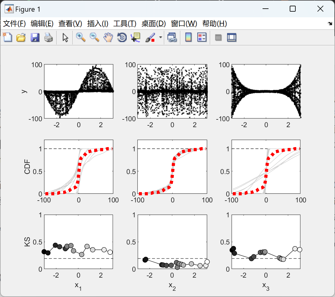
参数数量庞大是复杂环境模型面临的重要问题，限制了它们的应用。因此，敏感性分析（SA）方法旨在识别模型中的重要参数和非重要参数，可以对这些模型进行有效校准至关重要。敏感性分析确实通过应用因子固定（FF）和因子优先级排序（FP）来减少参与校准程序的参数数量。本文将基于密度的全局敏感性分析（GSA）方法-PAWN-应用于高参数化水文模拟器Soil and Water Assessment Tool（SWAT）。本研究旨在比较新开发的PAWN方法与广泛使用的方差敏感性分析方法Sobol’。PAWN方法考虑整个模型输出分布来描述输出的不确定性，而Sobol’方法隐含地假设方差是这一目的的充分指标。因此，选择了比利时齐南河（River Zenne）的SWAT模型中的26个与水量有关的参数，使用PAWN和Sobol’方法进行排名。此外，还评估和比较了这两种敏感性分析方法在收敛性、参数排名结果的演变以及所需计算成本等方面的表现。
关键词：全局敏感性分析，独立于矩的方法，基于方差的方法，SWAT模型

由于对物理过程的知识有所提高和计算能力的增强，过去几十年环境建模工具，如水文模拟器，变得更加复杂。此外，这些模型的应用也显著增加，特别是对于综合建模方法（Nossent等，2011；Shrestha等，2013）。然而，这样复杂的模拟器通常包含许多参数，其中大多数参数无法直接测量。因此，需要进行模型优化过程 - 即校准- 以估算参数值。为了获得高效的优化并避免过度参数化，敏感性分析（SA）对于识别模型的重要和非重要参数至关重要。敏感性分析确实可以减少校准中涉及的参数数量。这可以通过因子固定（FF）来实现，其中非重要参数被设置为固定值并从校准过程中排除，或者通过因子优先级排序（FP），其中更多关注放在对模型输出影响最大的参数上（Saltelli等人，2008）。

已经开发了许多不同的SA方法（Sobol’，1990；van Griensven等，2006；Borgonovo，2007）。读者可参考Saltelli等人（2000）以获取SA技术的详细描述。根据参数处理方式，SA方法分为两个主要分支，即局部方法和全局方法（Saltelli等人，2000）。局部技术在参数超空间的一个点评估灵敏度，而全局方法允许考虑整个参数范围（van Griensven等人，2006）。在存在参数不确定性的情况下，当难以为参数分配确定的值时，建议进行全局敏感性分析（GSA）（Saltelli等人，2002b）。GSA可以使用灵敏度指数（Saltelli，2002b）评估和量化不确定性源对模型输出不确定性的相对贡献。

📚2 运行结果

部分代码：

function [KS,xvals,y_u, y_c, par_u, par_c, ft] = PAWN(model, p, lb, ub, ...
Nu, n, Nc, npts, seed)
%PAWN Run PAWN for Global Sensitivity Analysis of a supplied model
%   [KS,xvals,y_u, y_c, par_u, par_c, ft] = PAWN(model, p, lb, ub, ...
% Nu, n, Nc, npts, seed)
%
%     model : A function that takes a vector of parameters x and a 
%             structure p as input to provide the model output as a scalar.
%             The vector holds parameters we need sensitivity of and p
%             holds all other parameters required to run the model.
%     lb : A vector (1xM) of the lower bounds for each parameter
%     ub : A vector (1xM) of the upper bounds for each parameter
%     Nu : Number of samples of the unconditioned parameter space
%     n : Number of conditioning values in each dimension
%     Nc : Number of samples of the conditioned parameter space
%     npts : Number of points to use in kernel density estimation
%     seed : Random number seed

    % Initializations
    M = length(lb); % Number of parameters
    y_u = nan(Nu,1); % Ouput of unconditioned simulations
    y_c = n * Nc * M; % Output of conditioned simulations
    KS = nan(M,n); % Kolmogorov-Smirnov statistic
    xvals = nan(M,n); % Container for conditioned samples
    ft = nan(M*n, npts); % CDF container
    
    rng(seed); % Set random seed
    % Containers for parameters
    par_u = bsxfun(@plus, lb, bsxfun(@times, rand(Nu, M), (ub-lb)));                 
    par_c = bsxfun(@plus, lb, bsxfun(@times, rand(M*Nc*n, length(lb)), (ub-lb)));
    % Create the conditioned samples
    for ind=1:M
        for ind2=1:n
            xvals(ind,ind2) = lb(ind) + rand*(ub(ind)-lb(ind));
            [(ind-1)*Nc*n+(ind2-1)*Nc+1:(ind-1)*Nc*n+ind2*Nc]
            par_c((ind-1)*Nc*n+(ind2-1)*Nc+1:...
                (ind-1)*Nc*n+ind2*Nc,ind) = xvals(ind,ind2);
        end
    end
    
    % Evaluate model output of unconditioned samples, can parallelize by
    % commenting out the parfor line and adding a comment to the for line.
%     parfor ind=1:Nu
    for ind=1:Nu
        y_u(ind) = model(par_u(ind,:), p);
    end
    
    % Evaluate model output of conditioned samples, can parallelize by
    % commenting out the parfor line and adding a comment to the for line.
%     parfor ind=1:length(par_c)
    for ind=1:length(par_c)
        y_c(ind) = model(par_c(ind,:), p);
    end
    
    % Find bounds of the model outputs
    m1 = min([y_c, y_u']);
    m2 = max([y_c, y_u']);
    % Evaluate the CDF with kernel density for unconditioned samples
    [f,~] = ksdensity(y_u, linspace(m1,m2,npts), 'Function', 'cdf');
    
    % Evaluate the CDF with kernel density for conditioned samples and use
    % that to find the KS statistic (Eqn 4 in the paper). 
    for ind=1:M
        for ind2=1:n
            % Temporarily store the current conditioned samples
            yt = y_c((ind-1)*Nc*n+(ind2-1)*Nc+1:(ind-1)*Nc*n+ind2*Nc);
            [ft((ind-1)*n+ind2,:),~] = ksdensity(yt, linspace(m1, m2,...
                                                 npts), 'Function', 'cdf');
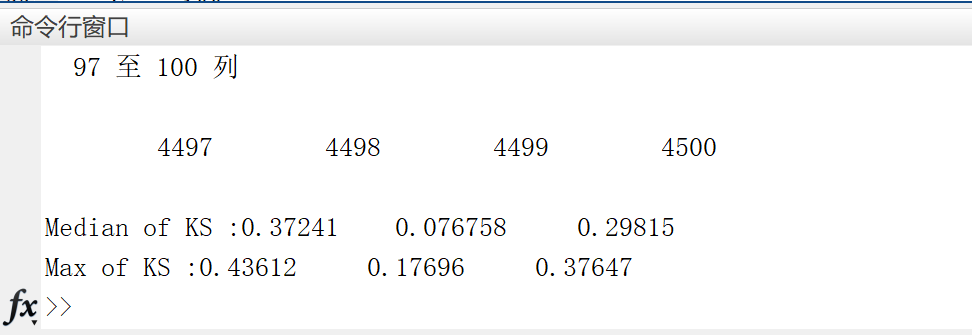
            KS(ind,ind2) = max(abs(ft((ind-1)*n+ind2,:)-f)); % Eqn 4
        end
    end
end

🎉3 参考文献

文章中一些内容引自网络，会注明出处或引用为参考文献，难免有未尽之处，如有不妥，请随时联系删除。

[1]: Pianosi, F., Wagener, T., 2015. A simple and efficient method for 
global sensitivity analysis based on cumulative distribution functions. 
Environ. Model. Softw. 67, 1-11. doi:10.1016/j.envsoft.2015.01.004

🌈4 Matlab代码、文献