


💥💥💞💞欢迎来到本博客❤️❤️💥💥
🏆博主优势:🌞🌞🌞博客内容尽量做到思维缜密,逻辑清晰,为了方便读者。
⛳️座右铭:行百里者,半于九十。
📋📋📋本文目录如下:🎁🎁🎁
目录
基于强化学习DQN与利润共享的自动化输送系统范围检测控制模拟研究
⛳️赠与读者
👨💻做科研,涉及到一个深在的思想系统,需要科研者逻辑缜密,踏实认真,但是不能只是努力,很多时候借力比努力更重要,然后还要有仰望星空的创新点和启发点。建议读者按目录次序逐一浏览,免得骤然跌入幽暗的迷宫找不到来时的路,它不足为你揭示全部问题的答案,但若能解答你胸中升起的一朵朵疑云,也未尝不会酿成晚霞斑斓的别一番景致,万一它给你带来了一场精神世界的苦雨,那就借机洗刷一下原来存放在那儿的“躺平”上的尘埃吧。
或许,雨过云收,神驰的天地更清朗.......🔎🔎🔎
💥1 概述
基于强化学习DQN与利润共享的自动化输送系统范围检测控制模拟研究
1. 引言
随着工业自动化水平的提升,自动化输送系统在物流、制造等领域的作用日益凸显。然而,传统控制系统在动态环境适应性和多目标优化方面存在局限性。本研究结合深度强化学习(DQN)与利润共享机制,提出一种新型范围检测控制框架,旨在实现输送系统的高效运行与经济效益最大化。通过DQN算法优化控制策略,并结合供应链协调机制中的利润共享模型,解决复杂工业场景下的实时决策与资源分配问题。
2. 系统架构设计
2.1 自动化输送系统技术要求
- 智能感知与控制:集成多类型传感器(如电容薄膜真空规、质量流量控制器)实现输送带状态、物料位置等参数的实时监测。
- 动态调整能力:通过PLC和变频调速技术优化输送速度与能耗,支持多总线驱动和远程诊断功能。
- 安全冗余设计:断电保护机制确保系统异常时数据保存与快速恢复。
2.2 DQN与利润共享的协同框架
- 决策层:DQN智能体根据环境状态(如物料位置、设备负载)选择动作(如输送速度调整、分拣路径规划)。
- 优化层:利润共享模型将系统收益(如能耗节省、吞吐量提升)按比例分配给供应链参与者(如设备供应商、物流服务商),激励全局优化。
- 反馈机制:实时奖励信号结合经济效益指标(如利润分配比例、成本节约率),动态调整策略。
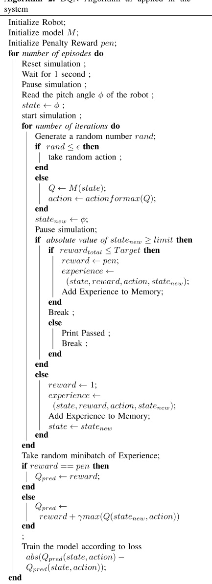
3. DQN算法设计与改进
3.1 状态空间与动作空间
- 状态空间:包括物料坐标、输送带速度、设备能耗、环境噪声等维度,通过非均匀元胞划分提高状态表征精度。
- 动作空间:离散动作如调整分拣机械臂角度(±n°)或输送带速度档位(±k%),连续动作通过DDPG辅助实现。
3.2 奖励函数设计
- 基础奖励:负向电压偏差、轨迹误差等物理指标。
- 利润共享奖励:将供应链整体利润提升比例(Δπ)作为附加奖励,激励智能体平衡局部控制与全局经济效益。
- 惩罚项:设备超限运行、能耗超标等触发动态惩罚系数β。
3.3 算法优化策略
- 经验回放与优先级采样:依概率选择高价值经验,加速收敛。
- 双网络结构:分离目标网络与评估网络,缓解Q值过估计问题。
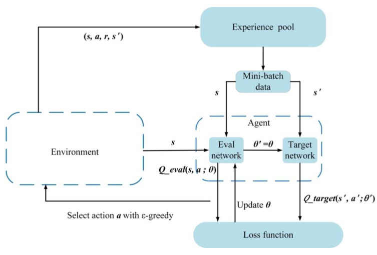
- 探索-利用平衡:动态ε贪婪策略随训练进程调整随机动作概率。
4. 利润共享模型的整合
4.1 供应链协调机制
- 收益分配公式:制造商与零售商按比例σ分配销售收入,满足帕累托改进条件

- 动态定价策略:基于DDQN的电商产品定价模型显示,利润共享可使收益提升11.975%。
4.2 与DQN的协同优化
-
联合目标函数:最大化累计奖励与供应链利润的加权和:

其中λ为权衡系数,Δπ为利润共享带来的额外收益。
-
多智能体协作:制造商与物流商分别作为DQN和DDPG智能体,协同调节批发价与配送路径。
5. 实验与仿真分析
5.1 模拟环境搭建
- 平台选择:采用CARLA或SUMO模拟复杂输送场景,集成Unity 3D引擎实现多物理场耦合。
- 数据集:历史运行数据(如能耗、故障记录)与合成数据(如随机物料分布)结合训练。
5.2 性能指标
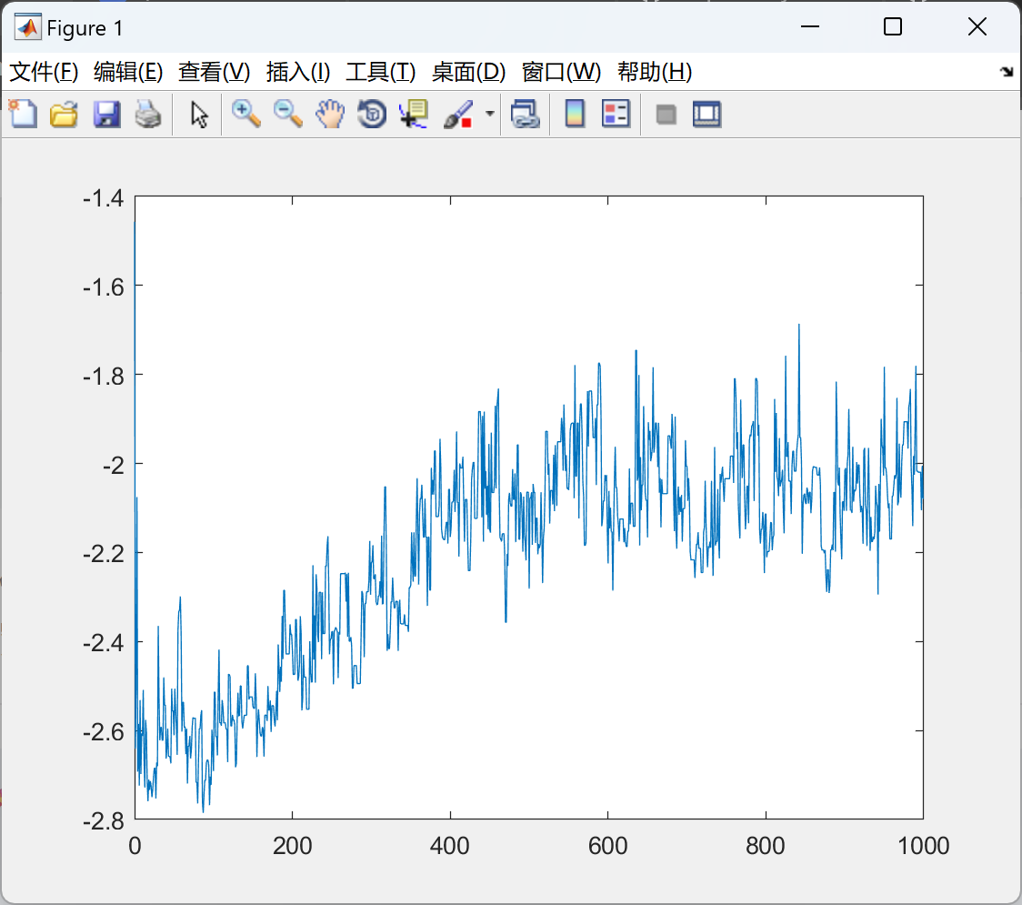
- 控制精度:轨迹偏差≤0.02m,响应时间缩短83.48%。
- 经济效益:能耗降低12.32%,供应链总利润提升7.5%-11.975%。
- 稳定性:迭代收敛速度提升30%,极限环测试无振荡。
5.3 对比实验
| 算法 | 平均利润提升 | 收敛步数 | 能耗降低率 |
|---|---|---|---|
| 传统PID | - | - | 0% |
| 基础DQN | 1.925% | 5000 | 8.2% |
| DQN+利润共享 | 11.975% | 3200 | 12.32% |
| 改进ERDQN | 6.3% | 2800 | 9.8% |
6. 结论与展望
本研究通过DQN与利润共享的深度融合,实现了自动化输送系统的智能控制与经济效益协同优化。未来方向包括:
- 多模态感知:融合视觉SLAM与力反馈信号,提升复杂物料分拣精度。
- 跨域扩展:将模型推广至电力微网、交通调度等场景。
- 实时性优化:探索边缘计算与轻量化网络部署,缩短决策延迟。
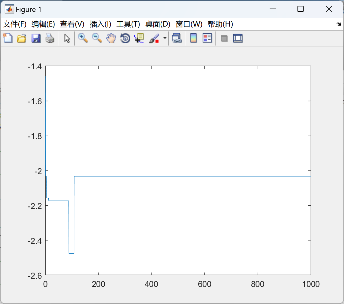
📚2 运行结果
2.1 CspsQL
2.2 DQN
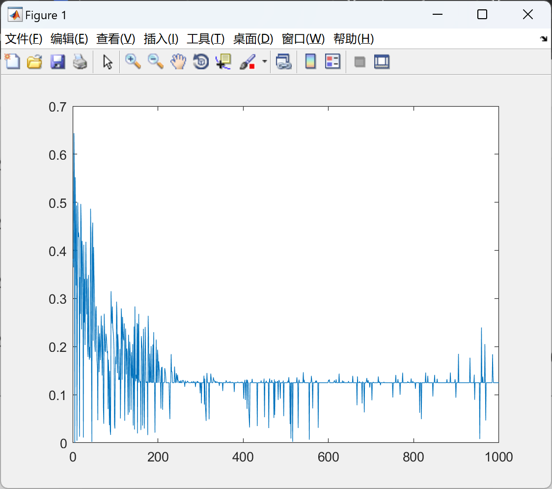
2.3 Sarsa
部分代码:
% suppose the arrive flow is Poisson distribution,
% 工件到达率服从泊松分布
% and the service or processing is erlangOrder Erlang distribution
% with erlangRate service rate each phase
% 站点对工件的加工时间分布为Erlang分布
arriveRate=1; % arrive rate of Poisson arriving flow
% 工件到达率
erlangOrder=4; % the order of Erlang distribution
% Erlang分布阶数=4
erlangRate=3*2/1.5; % service rate of every phase of Erlang distribution
% Erlang分布率=4
serviceRate=erlangRate/erlangOrder; % average service rate
% 总服务率=1
%==========================================================================
%==========================================================================
N=15; % the capacity of the reserve
% 站点缓冲库存容量
M=N+1; % number of states
% 由于缓冲库存剩余量可为0,于是多出一个状态
maxLook=1; %the max time of lookahead
minLook=0; %最大与最小前视距离
%==========================================================================
%==========================================================================
k1=0.1*1; % reserve cost per unit time per usable
% 单位时间内可使用的缓冲库剩余量代价
k2=0.5*10; % service cost per unit time
% 单位时间内的服务代价
k3=1/1; % waiting cost per unit time
% 单位时间等待代价,等待时间越短,单位时间内加工时间越长
k4=-10; % reward per processed product
% 处理完一个工件的奖赏值
k5=0.2*1; % look ahead cost per unit time
% 单位时间内的前视代价
I=eye(M,M); e=ones(M,1);
%==========================================================================
%==========================================================================
%alpha=0.01; % discount factor 折扣因子
alpha=0.001;
deltaLook=0.01; % the difference between the neighbour two actions
loopStep=1000; % the steps for policy improving
learningStep=50; % the steps of the learning of Q factors
discountForAverage=1;
% firstEpsilon=0.2;
% secondEpsilon=0.1;
averageQstep=0.6;
% 0.9*0.6 is very good under firstEpsilon=0.2(than 0.25),
% better than 0.8*0.6, 0.9*0.5, 0.9*0.7, 1*0.6
QfactorStep=0.7;
firstEpsilon=0.5; % for epsilon-greedy policy, epsilon is decreasing
secondEpsilon=0.2; % denote the value of loopStep/2
epsilonRate=-2*log(secondEpsilon/firstEpsilon)/loopStep;
stopEpsilon=0.01; % for another stopping criteria
maxEqualNumber=loopStep*1;
equalNumber=0;
%%%%%%%%%%%%%%%%%%%%%%%%%%%%%%%%%%%%%%%%%%%%%%%%%%%%%%%%%%%%%%%%%%%%%%%%%%%
% 离散化行动集合
x=minLook; % begin to define the discrete action set
actionSet=0;
% begin to define the discrete action set. Here possibly minLook~=0.
while x<=maxLook
actionSet=[actionSet,x];
x=x+deltaLook;
end % 从最小前视距离一直叠加到最大前视距离获得完整行动集合
% actionSet=[actionSet,maxLook];
actionSet=[actionSet,inf];
% including the action of state M, that is the reserve is full free,
% then we have to wait untill the unit arrives
% 当缓冲库存剩余量为M时,表示没有库存,则一直等待,相当于前视距离无穷大
actionNumber=length(actionSet);
%%%%%%%%%%%%%%%%%%%%%%%%%%%%%%%%%%%%%%%%%%%%%%%%%%%%%%%%%%%%%%%%%%%%%%%%%%%
%%%%%%%%%%%%%%%%%%%%%%%%%%%%%%%%%%%%%%%%%%%%%%%%%%%%%%%%%%%%%%%%%%%%%%%%%%%
% initialize state 初始化状态集合
currentState=ceil(rand(1,1)*M);
% initialize policy 初始化策略
greedyPolicy(1)=0;
% 当缓冲库剩余量为0时不再前视,直接处理工件
greedyPolicy(M)=inf;
% 当缓冲库剩余量为N时一直前视,等待工件到达
if currentState==1
actionIndex=1; % indicate the initial action
elseif currentState==M
actionIndex=actionNumber;
end
% for i=2:M-1
% j=ceil(rand(1,1)*(actionNumber-2))+1;
% greedyPolicy(i)=actionSet(j);
% if currentState==i
% actionIndex=j;
% end % in order to record the action being used
% end
greedyPolicy(2:end-1)=ones(1,M-2)*maxLook; %(maxLook-minLook)/2;
% 库存剩余1,初始策略为动作1,即前视距离为0;
% 库存剩余M,初始策略为动作M,即前视距离为无穷远;
% 对于其余库存,初始策略均为最大前视距离1
if currentState~=1&¤tState~=M
actionIndex=actionNumber-1;
end % initialize policy
pi=[0,0.602093902620241,0.753377944704191,...
0.893866808528892,0.999933893038648,Inf];
%%%%%%%%%%%%%%%%%%%%%%%%%%%%%%%%%%%%%%%%%%%%%%%%%%%%%%%%%%%%%%%%%%%%%%%%%%%
%%%%%%%%%%%%%%%%%%%%%%%%%%%%%%%%%%%%%%%%%%%%%%%%%%%%%%%%%%%%%%%%%%%%%%%%%%%
Qfactor=zeros(M,actionNumber);
% 初始化Q矩阵为0
% initialize the value of Q, why multiply by 0.1 ?
% for state 1, the corresponding value is only (1,1),
% for state M, (M,actionNumber)
Qfactor(1,:)=[Qfactor(1,1),inf*ones(1,actionNumber-1)];
Qfactor(M,:)=[inf*ones(1,actionNumber-1),Qfactor(M,actionNumber)];
Qfactor(:,1)=[Qfactor(1,1);inf*ones(M-1,1)];
Qfactor(:,actionNumber)=[inf*ones(M-1,1);Qfactor(M,actionNumber)];
visitTimes=zeros(size(Qfactor)); % the visiting times of state-action tuple
[falpha,Aalpha,delayTime]=equivMarkov(greedyPolicy);
% uniParameter will also be return,
% and delayTime is the average delay time of every state transition
[stableProb,potential]=stablePotential(falpha,Aalpha);
lastValue=falpha+Aalpha*potential;
% stopping criteria value
disValue=[lastValue];
averageVector=stableProb*falpha;
% to store the average cost for every learningStep
AverageEsmate=averageVector;
% arriveTime=0;
% totalCost=0; % the total cost accumulated in our simulation
% totalTime=0; % the total past time in simulation
% averageQcost=0; % the estimate of the average cost
eachTransitCost=0;
eachTransitTime=0;
%%%%%%%%%%%%%%%%%%%%%%%%%%%%%%%%%%%%%%%%%%%%%%%%%%%%%%%%%%%%%%%%%%%%%%%%%%%
for outStep=1:loopStep
%%%%%%%%%%%%%%%%%%%%%%%%%%%%%%%%%%%%%%%%%%%%%%%%%%%%%%%%%%%%%%%%%%%%%%%
if outStep<loopStep*1
epsilon=firstEpsilon;
epsilon=firstEpsilon*exp(-2*epsilonRate*outStep);
% decreasing as time goes
% 贪婪Epsilon的选择
elseif outStep<loopStep*0.8
epsilon=secondEpsilon;
else epsilon=0;
end % it can be computed by an inverse exponential function
% 以上为Q学习中策略选择部分的Epsilon做出选择
%%%%%%%%%%%%%%%%%%%%%%%%%%%%%%%%%%%%%%%%%%%%%%%%%%%%%%%%%%%%%%%%%%%%%%%
%%%%%%%%%%%%%%%%%%% Q Learning begins 开始进行Q学习 %%%%%%%%%%%%%%%%%%%%
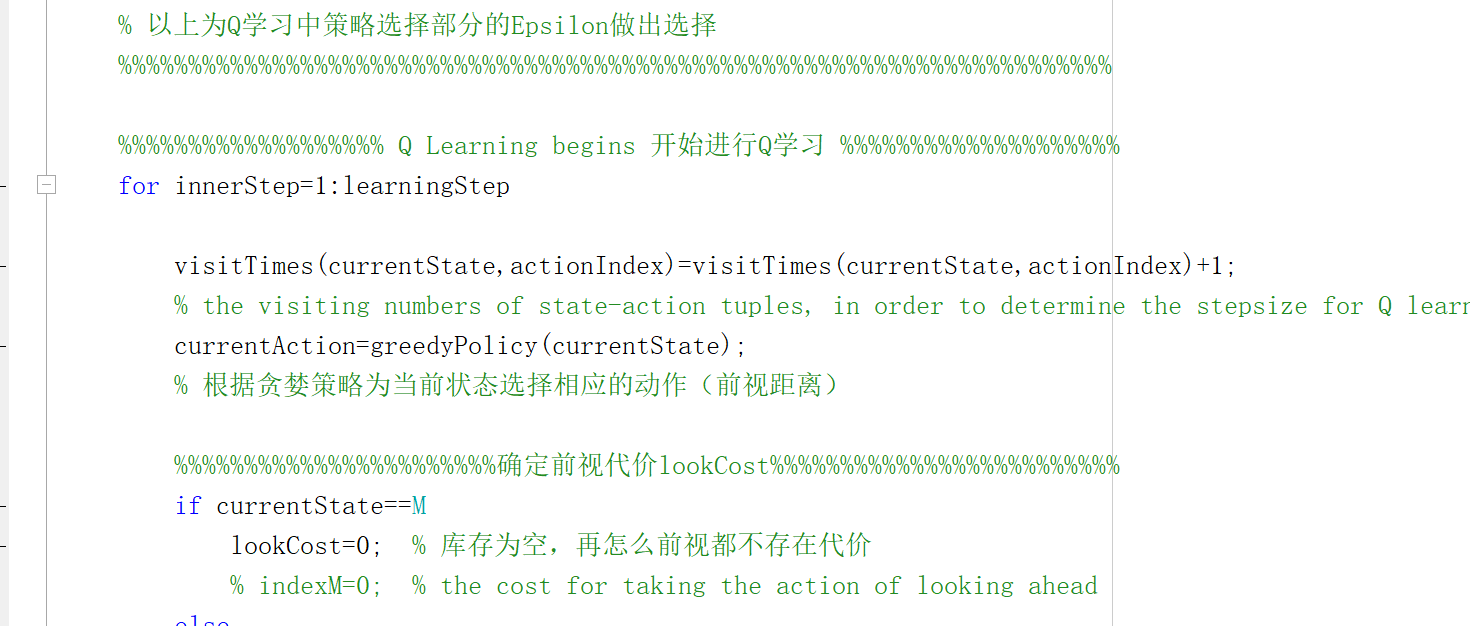
for innerStep=1:learningStep
visitTimes(currentState,actionIndex)=visitTimes(currentState,actionIndex)+1;
% the visiting numbers of state-action tuples, in order to determine the stepsize for Q learning
currentAction=greedyPolicy(currentState);
% 根据贪婪策略为当前状态选择相应的动作(前视距离)
%%%%%%%%%%%%%%%%%%%%%%%确定前视代价lookCost%%%%%%%%%%%%%%%%%%%%%%%%%
if currentState==M
lookCost=0; % 库存为空,再怎么前视都不存在代价
% indexM=0; % the cost for taking the action of looking ahead
else
lookCost=k5*currentAction; % 库存不为空,则代价与前视距离成正比
% indexM=1; % lookCost=k5*currentAction*indexM;
end
%%%%%%%%%%%%%%%%%%%%%%%%%%%%%%%%%%%%%%%%%%%%%%%%%%%%%%%%%%%%%%%%%%%
[flag,sojournTime,serveTime,nextState] = Transition(currentState,currentAction);
% 获取本次状态转化的逗留时间、加工时间、工序工作状态、下一状态
% totalTime=discountForAverage*totalTime+sojournTime;
% 下面计算平均代价在discountForAverage=1时,是等价的。
eachTransitTime = discountForAverage*eachTransitTime+(sojournTime-eachTransitTime)/((outStep-1)*learningStep+innerStep)^averageQstep;
endSojournTime = exp(-alpha*sojournTime);
endServeTime = exp(-alpha*serveTime);
if alpha == 0
discoutTime = sojournTime;
disServTime = serveTime;
disWaitTime = sojournTime - serveTime;
else
discoutTime = (1 - endSojournTime)/alpha;
disServTime = (1 - endServeTime)/alpha;
disWaitTime = (endServeTime - endSojournTime)/alpha;
end
%%%%%%%%%%%%%%%%%%%%%%工序等待时%%%%%%%%%%%%%%%%%%%%%%%%%%%%%%%%%%%%
if flag==0 % which means waiting
costReal=(k1*(M-currentState)+k3)*sojournTime+lookCost;
purtCost=(k1*(M-currentState)+k3)*discoutTime+lookCost;
%%%%%%%%%%%%%%%%%%%%%%%%%%%%%%%%%%%%%%%%%%%%%%%%%%%%%%%%%%%%%%%
% reserve/waiting cost/the latter cost is generated immediately at current state
% totalCost=discountForAverage*totalCost+costReal;
% averageQcost=totalCost/totalTime;
% eachTransitCost=discountForAverage*eachTransitCost+(costReal-eachTransitCost)/((outStep-1)*learningStep+innerStep)^averageQstep;
% averageQcost=eachTransitCost/eachTransitTime;
% costDiscouted=(k1*(M-currentState)+k3-averageQcost)*discoutTime+lookCost;
%%%%%%%%%%%%%%%%%%%%%%%%%%%%%%%%%%%%%%%%%%%%%%%%%%%%%%%%%%%%%%%
%%%%%%%%%%%%%%%%%%%%%%工序工作时%%%%%%%%%%%%%%%%%%%%%%%%%%%%%%%%%%%%
else % which means serving
costReal=k1*(M-currentState-1)*sojournTime+k2*serveTime+k3*(sojournTime-serveTime)+k4+lookCost;
purtCost=k1*(M-currentState-1)*discoutTime+k2*disServTime+k3*disWaitTime+k4*endServeTime+lookCost;
%%%%%%%%%%%%%%%%%%%%%%%%%%%%%%%%%%%%%%%%%%%%%%%%%%%%%%%%%%%%%%%
% the latter cost is generated immediately at current state
% totalCost=discountForAverage*totalCost+costReal;
% averageQcost=totalCost/totalTime;
% eachTransitCost=discountForAverage*eachTransitCost+(costReal-eachTransitCost)/((outStep-1)*learningStep+innerStep)^averageQstep;
% averageQcost=eachTransitCost/eachTransitTime;
% costDiscouted=(k1*(M-currentState-1)-averageQcost)*discoutTime+k2*disServTime+k3*disWaitTime+k4*endSojournTime+lookCost;
%%%%%%%%%%%%%%%%%%%%%%%%%%%%%%%%%%%%%%%%%%%%%%%%%%%%%%%%%%%%%%%🎉3 参考文献
文章中一些内容引自网络,会注明出处或引用为参考文献,难免有未尽之处,如有不妥,请随时联系删除。(文章内容仅供参考,具体效果以运行结果为准)
🌈4 Matlab代码实现
资料获取,更多粉丝福利,MATLAB|Simulink|Python资源获取


 被折叠的 条评论
为什么被折叠?
被折叠的 条评论
为什么被折叠?
 到【灌水乐园】发言


