Free Energy Calculations: Methane in Water自由能计算：甲烷在水中的情况

Free Energy Calculations: Methane in Water
自由能计算：甲烷在水中的情况

Justin A. Lemkul, Ph.D.  贾斯汀·A·勒姆库尔，博士
Virginia Tech Department of Biochemistry
弗吉尼亚理工大学生物化学系

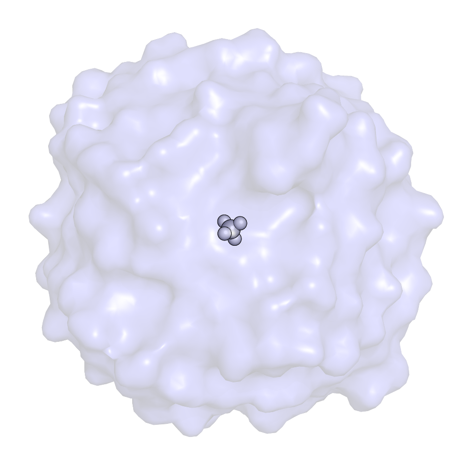
This tutorial will guide the user through the process of calculating a simple free energy change, the decoupling removal of van der Waals interactions between neutral methane and a box of water. This quantity was previously calculated by Shirts et al. in a systematic evaluation of free energies of solvation of amino acid side chains using different atomistic force fields. 本教程将指导用户计算一个简单的自由能变化，即在中性甲烷和水箱之间解耦去除范德华相互作用。该量先前由 Shirts 等人使用不同的原子力场系统地评估氨基酸侧链的溶剂化自由能时计算过。 This tutorial requires a GROMACS version in the 2018.x series. 本教程需要使用 2018.x 系列的 GROMACS 版本。

Step One: Theory  第一步：理论

This tutorial will assume you have a reasonable understanding of what free energy calculations are, the different types that exist, and the underlying theory of the technique. It is neither practical nor possible to provide a complete education here. Instead, I will focus this tutorial on practical aspects of running free energy calculations in GROMACS, highlighting relevant theoretical points as necessary throughout the tutorial. I will provide here a list of useful papers for those who are new to free energy calculations. Do not consider this list exhaustive. It should also not supplant proper study of statistical mechanics and the many books and papers that have been written on related topics. 本教程将假设您对自由能计算有合理的理解，包括存在的不同类型以及该技术的理论基础。在这里提供完整的教育既不实用也不可能。相反，我将本教程的重点放在 GROMACS 中运行自由能计算的实用方面，并在教程中根据需要强调相关的理论要点。我将为自由能计算的新手提供一份有用的论文列表。请勿认为这份列表是详尽的。它也不应取代对统计力学的深入学习，以及许多已撰写的相关主题的书籍和论文。 C. D. Christ, A. E. Mark, and W. F. van Gunsteren (2010) J. Comput. Chem. 31: 1569-1582. C. D. Christ, A. E. Mark, 和 W. F. van Gunsteren (2010) : 1569-1582.DOI C. D. Christ, A. E. Mark, 和 W. F. van Gunsteren (2010) J. Comput. Chem. 31: 1569-1582. DOI A. Pohorille, C. Jarzynski, and C. Chipot (2010) J. Phys. Chem. B 114: 10235-10253. A. Pohorille, C. Jarzynski, 和 C. Chipot (2010) : 10235-10253.DOI A. Pohorille, C. Jarzynski, 和 C. Chipot (2010) J. Phys. Chem. B 114: 10235-10253. DOI A. Villa and A. E. Mark (2002) J. Comput. Chem. 23: 548-553. A. Villa 和 A. E. Mark (2002) : 548-553.DOI A. Villa 和 A. E. Mark (2002) J. Comput. Chem. 23: 548-553. DOI  The objective of this tutorial is to reproduce the results of a very simple system for which an accurate free energy estimate exists. The system of choice (methane in water) is one dealt with by Shirts et al. in a systematic study of force fields and the free energies of hydration of amino acid side chain analogs. The complete publication can be found here. This tutorial will assume you have read and understood the broader points of this paper. 本教程的目的是重现一个简单系统的结果，该系统具有准确的自由能估计值。所选系统（水中的甲烷）是 Shirts 等人系统研究力场和氨基酸侧链类似物水合自由能时处理过的。完整的出版物可在此处找到。本教程假定你已经阅读并理解了这篇论文的更广泛要点。 Rather than use the thermodynamic integration approach for evaluating free energy differences, the data analysis conducted here will utilize the GROMACS "bar" module, which was introduced in GROMACS version 4.5 (and previously called g_bar). It uses the Bennett Acceptance Ratio (BAR, hence the name of the module) method for calculating free energy differences. The corresponding paper for BAR can be found here. Knowledge of this method is also assumed and will not be discussed in great detail here. 这里将不使用热力学积分方法来评估自由能差异，而将采用 GROMACS 的"bar"模块进行数据分析，该模块于 GROMACS 4.5 版本中引入（此前被称为 g_bar）。它使用 Bennett 接受比（BAR，这也是该模块名称的由来）方法来计算自由能差异。BAR 的相关论文可在此处找到。也假定你对这种方法有所了解，因此在这里不会详细讨论。 Free energy calculations have a number of practical applications, of which some of the more common ones include free energies of solvation/hydration and free energy of binding for a small molecule to some larger receptor biomolecule (usually a protein). Both of these procedures involve the need to either add (introduce/couple) or remove (decouple/annihilate) the small molecule of interest from the system and calculate the resulting free energy change. 自由能计算有许多实际应用，其中一些较常见的包括小分子与较大受体生物分子（通常是蛋白质）的溶剂化/水合自由能和结合自由能。这两种方法都需要将目标小分子添加（引入/耦合）到系统中或从系统中移除（解耦/湮灭），并计算由此产生的自由能变化。 There are two types of nonbonded interactions that can be transformed during free energy calculations, Coulombic and van der Waals interactions. Bonded interactions can also be manipulated, but for simplicity, will not be addressed here. For this tutorial, we will calculate the free energy of a very simple process: turning off the Lennard-Jones interactions between the atomic sites of a molecule of interest (in this case, methane) in water. This quantity was calculated very precisely by Shirts et al. and thus it is the quantity we seek to reproduce here. 在自由能计算中，可以转换两种非键相互作用：库仑相互作用和范德华相互作用。键相互作用也可以进行操作，但为简化起见，这里不予以讨论。在本教程中，我们将计算一个非常简单过程的自由能：关闭目标分子（在本例中为甲烷）在水中原子位点之间的 Lennard-Jones 相互作用。该量由 Shirts 等人非常精确地计算过，因此这是我们在此处寻求重现的量。

Step Two: Examine the Topology
第二步：检查拓扑结构

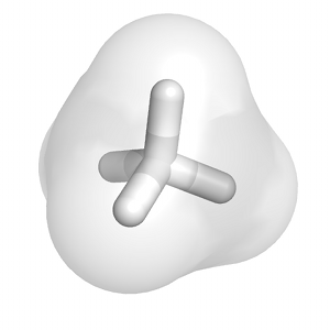
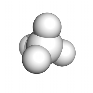
Download the coordinate file and topology for this system. These files were provided as part of David Mobley's tutorial for this system (which is no longer online), and are the original files (modified slightly for compatibility with recent GROMACS versions) used by Michael Shirts in the paper referenced on the previous page. 下载该系统的坐标文件和拓扑文件。这些文件是 David Mobley 为该系统提供的教程的一部分（该教程现已不再在线），并且是 Michael Shirts 在上一页引用的论文中使用的原始文件（为兼容较新的 GROMACS 版本稍作修改）。 The system contains a single molecule of methane (called "ALAB" in the coordinate file, for the β-carbon of alanine) in a box of 596 TIP3P water molecules. Looking into the topology, we find: 该系统包含一个甲烷分子（在坐标文件中称为"ALAB"，代表丙氨酸的β-碳）在一个由 596 个 TIP3P 水分子组成的盒子中。查看拓扑结构，我们发现： ; Topology for methane in TIP3P #include "oplsaa.ff/forcefield.itp" [ moleculetype ] ; Name nrexcl Methane 3 [ atoms ] ; nr type resnr residue atom cgnr charge mass typeB chargeB massB 1 opls_138 1 ALAB CB 1 0.000 12.011 2 opls_140 1 ALAB HB1 2 0.000 1.008 3 opls_140 1 ALAB HB2 3 0.000 1.008 4 opls_140 1 ALAB HB3 4 0.000 1.008 5 opls_140 1 ALAB HB4 5 0.000 1.008 [ bonds ] ; ai aj funct c0 c1 c2 c3 1 2 1 1 3 1 1 4 1 1 5 1 [ angles ] ; ai aj ak funct c0 c1 c2 c3 2 1 3 1 2 1 4 1 2 1 5 1 3 1 4 1 3 1 5 1 4 1 5 1 ; water topology #include "oplsaa.ff/tip3p.itp" [ system ] ; Name Methane in water [ molecules ] ; Compound #mols Methane 1 SOL 596 You will note that all charges are set to zero. There is a practial reason behind this setup. Normally, charge interactions between the solute and water are turned off prior to the van der Waals terms. If charge interactions are left on when Lennard-Jones terms are turned off, positive and negative charges would be allowed to approach one another at infinitely close distances, resulting in a very unstable system that would probably just blow up. The procedure in this tutorial essentially assumes that charges have been properly been turned off prior to this point, and we will be turning off only van der Waals interactions between the solute and solvent. 您会注意到所有电荷都被设置为零。这种设置背后有一个实际原因。通常，在范德华项之前，溶剂和溶质之间的电荷相互作用会被关闭。如果当范德华项关闭时仍然保留电荷相互作用，正负电荷会被允许在无限接近的距离上相互接近，导致系统非常不稳定，可能会直接爆炸。本教程中的步骤基本上假设在这一点之前电荷已经被正确关闭，我们将只关闭溶质和溶剂之间的范德华相互作用。 Note that in previous versions of GROMACS, the contents of the typeB, chargeB, and massB headings had to correspond to a B-state of the molecule. As of GROMACS version 4.0, topology modifications for simple (de)couplings are no longer required (hooray!), but in the case of mutating one molecule to another, wherein bonded and nonbonded terms may change, the old-style modifications (the so-called "dual topology approach") would still be required. The GROMACS manual, section 5.8.4, provides an example of such a transformation. 请注意，在 GROMACS 的早期版本中， typeB 、 chargeB 和 massB 标题的内容必须对应分子的 B 态。自 GROMACS 4.0 版本起，对于简单的（解）耦合，拓扑修改不再需要（太好了！），但在将一种分子转变为另一种分子的情况下，其中键合和非键合项可能会发生变化，仍然需要使用旧式的修改（所谓的"双重拓扑方法"）。GROMACS 手册第 5.8.4 节提供了一个此类转换的示例。

Step Three: The Workflow  第三步：工作流程

The free energy change of transforming a system from state A to state B, ΔGAB, is a function of a coupling parameter, λ, which indicates the level of change that has taken place between states A and B, that is, the extent to which the Hamiltonian has been perturbed and the system has been transformed. Simulations conducted at different values of λ allow us to plot a ∂H/∂λ curve, from which ΔGAB is derived. The first step in planning free energy calculations is how many λ points will be used to describe the transformation from state A (λ = 0) to state B (λ = 1), with the goal of collecting adequate data to exhaustively sample phase space and produce a reliable ∂H/∂λ curve. 将系统从状态 A 转变为状态 B 的自由能变化ΔG AB 是一个耦合参数λ的函数，λ表示状态 A 和状态 B 之间发生的变化程度，即哈密顿量扰动和系统转化的程度。在不同λ值下进行的模拟使我们能够绘制出∂H/∂λ曲线，从而得到ΔG AB 。规划自由能计算的第一步是确定将使用多少个λ点来描述从状态 A（λ = 0）到状态 B（λ = 1）的转化，目标是收集足够的数据以充分采样相空间并生成可靠的∂H/∂λ曲线。 λ = 0 λ = 0.5 λ = 1 For decoupling Coulombic interactions, which depend linearly upon λ, an equidistant λ spacing from 0 to 1 should usually suffice, with λ spacing values of of 0.05-0.1 being common. Note that this is a broad generalization, and in fact many molecules will require a great deal more finesse, such as those that interact very strongly with the surrounding environment through hydrogen bonding. In this case, λ spacing may need to be decreased, such that more points are used, perhaps even in an asymmetric fashion. 为了解耦依赖于λ的库仑相互作用，通常使用从 0 到 1 的等距λ间隔就足够了，常见的λ间隔值为 0.05-0.1。请注意，这是一种广泛的概括，实际上许多分子需要更多的技巧，例如那些通过氢键与周围环境强烈相互作用的分子。在这种情况下，λ间隔可能需要减小，使用更多的点，甚至可能采用非对称的方式。 For decoupling van der Waals interactions, λ spacing can be much trickier. For reasons described by Shirts et al. and elsewhere, a great deal of λ points may be necessary to properly describe the transformation. Clustering λ points in regions where the slope of the ∂H/∂λ curve is steep may be necessary. For the purposes of this tutorial, we will use equidistant λ spacing of 0.05, but in many cases, one may need to use different spacing, especially clustering values in the range of 0.6 ≤ λ ≤ 0.8. 为了解耦范德华相互作用，λ间隔可能更加复杂。根据 Shirts 等人及其他文献中的描述，可能需要大量的λ点来正确描述这种转换。可能需要在∂H/∂λ曲线斜率较大的区域聚集λ点。在本教程中，我们将使用 0.05 的等距λ间隔，但在许多情况下，可能需要使用不同的间隔，特别是在 0.6 ≤ λ ≤ 0.8 的范围内聚集值。 For each value of λ, a complete workflow (energy minimization, equilibration, and data collection) must be conducted. I generally find it most efficient to run these jobs as batches, passing the output of one step directly into the next. The workflow utilized here will be: 对于每个λ值，必须执行一个完整的流程（能量最小化、平衡和数据分析）。我通常发现将这些任务作为批次运行最有效率，将一个步骤的输出直接传递到下一个步骤。这里使用的流程将是： Steepest descents minimization 最速下降最小化 NVT equilibration   NVT 平衡 NPT equilibration   NPT 平衡 Data collection under an NPT ensemble 在 NPT 系综下收集数据 The .mdp files for the different steps of the tutorial (for λ = 0 only) are provided at the following links: 教程的不同步骤（仅λ = 0）的.mdp 文件提供在以下链接： Steepest descents EM  最速下降 EM NVT equilibration  NVT 平衡 NPT equilibration  NPT 平衡 Production MD  生产 MD I am also making available an accessory Perl script, write_mdp.pl, that you can use to very quickly produce all of the input files needed for running these simulations. 我还提供了一个辅助的 Perl 脚本 write_mdp.pl，你可以用它非常快速地生成运行这些模拟所需的所有输入文件。 You can also download a shell script (job.sh) for running these jobs according to the workflow I will describe. 你还可以下载一个 shell 脚本（job.sh），用于根据我将描述的工作流程运行这些作业。 If you issue:  如果你执行： perl write_mdp.pl em_steep.mdp You will receive files named em_steep_0.mdp, em_steep_1.mdp, ... em_steep_20.mdp, with the relevant values of init_lambda_state inserted into the filename. Analogously, you can produce the rest of your .mdp files in the same way (nvt.mdp, npt.mdp, and md.mdp). 你将获得文件名 em_steep_0.mdp、em_steep_1.mdp、...、em_steep_20.mdp，文件名中插入了 init_lambda_state 的相关值。类似地，你可以以相同的方式生成其余的.mdp 文件（nvt.mdp、npt.mdp 和 md.mdp）。 In job.sh, you will need to change the values of $FREE_ENERGY and $MDP, otherwise the script certainly won't work. 在 job.sh 中，你需要更改 $FREE_ENERGY 和 $MDP 的值，否则脚本肯定无法工作。   Notes on .mdp settings .mdp 设置的注意事项 Before proceeding, it is important to understand the free energy-related settings in the .mdp files (using em_steep_0.mdp as an example). They are the same for all steps in the workflow. I will assume that you are familiar with the other settings found in the .mdp file. If this is not the case, please refer to some more basic tutorial material before proceeding. 在进行下一步之前，了解.mdp 文件中的自由能相关设置非常重要（以 em_steep_0.mdp 为例）。这些设置在所有工作流程步骤中都是相同的。我将假设您熟悉.mdp 文件中的其他设置。如果情况并非如此，请在继续之前参考一些更基础的教程材料。 free_energy = yes Indicates that we are doing a free energy calculation, and that interpolation between the A and B states of the chosen molecule (defined below) will occur. 表示我们正在进行自由能计算，并且将在所选分子（定义如下）的 A 和 B 状态之间进行插值。 init_lambda_state = 0 In previous GROMACS versions, the "init_lambda" keyword specified a single value of λ directly. Since version 5.0, λ is now a vector that allows for transformation of bonded and nonbonded interactions. With the init_lambda_state keyword, we specify an index (starting from zero) of the vector to be utilized in the simulation (more on this later). 在之前的 GROMACS 版本中，"init_lambda"关键字直接指定了一个λ的单一值。自 5.0 版本起，λ现在是一个向量，允许对键合和非键合相互作用进行转换。通过 init_lambda_state 关键字，我们指定在模拟中要使用的向量的索引（从零开始）（更多内容将在后面介绍）。 delta_lambda = 0 The value of λ can be incremented by some amount per timestep (i.e., δλ/δt) in a technique called "slow growth." This method can have significant errors associated with it, and thus we will make no time-dependent changes to our λ values. λ的值可以通过每个时间步长增加一定的量（即δλ/δt）在一种称为"慢增长"的技术中实现。这种方法与其相关联的显著误差，因此我们将不对我们的λ值进行时间相关的改变。 fep_lambdas = (nothing) You will note that this keyword is not specified. In previous GROMACS versions, the use of init_lambda and foreign_lambda controlled the value of λi and the additional values of λ for which energy differences would be evaluated for configurations at λi. This is no longer the case. One can explicitly set values of λ in the fep_lambdas keyword, but instead we allow the calc_lambda_neighbors keyword (see below) to automatically determine these additional values. 您会注意到这个关键字没有指定。在之前的 GROMACS 版本中，init_lambda 和 foreign_lambda 的使用控制了λ的值以及λ的附加值，这些附加值用于计算λ状态下配置的能量差。现在情况不再如此。用户可以在 fep_lambdas 关键字中显式设置λ的值，但我们允许 calc_lambda_neighbors 关键字（见下文）自动确定这些附加值。 calc_lambda_neighbors = 1 The number of neighboring windows for which energy differences are computed with respect to λi. For instance, if init_lambda_state is set to 10, then energy differences with respect to λ states 9 and 11 are computed during the run with calc_lambda_neighbors = 1. 用于计算与λ相关的能量差的相邻窗口数量。例如，如果 init_lambda_state 设置为 10，那么在 calc_lambda_neighbors = 1 的情况下，会计算λ状态 9 和 11 的能量差。 vdw_lambdas = ... An array of λ values for the transformation of van der Waals interactions. van der Waals 相互作用的λ值数组。 coul_lambdas = ... An array of λ values for the transformation of Coulombic (electrostatic) interactions. Coulombic（静电）相互作用的λ值数组。 bonded_lambdas = ... An array of λ values for the transformation of bonded interactions. 用于键合相互作用转换的λ值数组。 restraint_lambdas = ... An array of λ values for the transformation of restraints. 用于约束转换的λ值数组。 mass_lambdas = ... An array of λ values for the transformation of atomic masses; used if tranforming the chemical nature of the molecule. 用于原子质量转换的一系列λ值；如果转换分子的化学性质时使用。 temperature_lambdas = ... An array of λ values for the transformation of temperatures; used only for simulated tempering. 用于温度转换的一系列λ值；仅用于模拟退火。 sc-alpha = 0.5 The value of the α scaling factor used in the "soft-core" Lennard-Jones equation. See equations 4.124 - 4.126 in the GROMACS manual, section 4.5.1, for a complete description of this term, as well as the next three. α缩放因子在"软核"伦纳德-琼斯方程中的值。有关该术语以及接下来三个术语的完整描述，请参阅 GROMACS 手册第 4.5.1 节中的公式 4.124 至 4.126。 sc-coul = no Transform Coulombic interactions linearly. This is the default behavior, but is written out for clarity. 线性转换库仑相互作用。这是默认行为，但为了清晰起见，这里明确写出。 sc-power = 1.0 The power for λ in the soft-core equation. λ在软核方程中的幂。 sc-sigma = 0.3 The value of σ assigned to any atom types that have C6 or C12 parameters equal to zero or σ < sc-sigma (typically H atoms). This value is used in the soft-core Lennard-Jones equation. 为任何具有 C6 或 C12 参数等于零或σ < sc-sigma 的原子类型分配的σ值（通常为 H 原子）。此值用于软核 Lennard-Jones 方程。 couple-moltype = Methane The name of the [moleculetype] in that will have its topology interpolated from state A to state B. Note that the name given here must match a [moleculetype] name, and not the residue name. In some cases these may be the same, but I have maintained different names for the [moleculetype] and component residue for instructive purposes. 那个[moleculetype]的名称将从状态 A 插值到状态 B。请注意，这里提供的名称必须与[moleculetype]名称匹配，而不是残基名称。在某些情况下它们可能是相同的，但我为了说明目的，为[moleculetype]和组件残基保留了不同的名称。 couple-lambda0 = vdw The types of nonbonded interactions that are present in state A between the interpolated [moleculetype] and the remainder of the system. The value "vdw" indicates that only van der Waals terms are active between methane and water; there are no solute-solvent Coulombic interactions. 在状态 A 中，插值[moleculetype]与系统其余部分之间的非键合相互作用类型。值"vdw"表示甲烷和水之间仅激活范德华项；没有溶质-溶剂库仑相互作用。 couple-lambda1 = none The types of nonbonded interactions that are present in state B between the interpolated [moleculetype] and the remainder of the system. The value "none" indicates that both van der Waals and Coulombic interactions are off in state B. Relative to couple-lambda0, this indicates that only van der Waals terms have been turned off. 在状态 B 中，插值[moleculetype]与系统其余部分之间的非键相互作用类型。"none"值表示在状态 B 中范德华力和库仑力均关闭。相对于 couple-lambda0，这表示仅关闭了范德华力项。 couple-intramol = no Do not decouple intramolecular interactions. That is, the λ factor is applied to only solute-solvent nonbonded interactions and not solute-solute nonbonded interactions. 不要解耦分子内相互作用。也就是说，λ因子仅应用于溶质-溶剂非键相互作用，而不应用于溶质-溶质非键相互作用。 Setting "couple-intramol = yes" is useful for larger molecules that may have intramolecular interactions occuring at longer distance (e.g. peptides or other polymers). Otherwise, distal parts of the molecule will interact via explicit pair interactions in an unnaturally strong manner (since solute-solvent interactions are weakened as a function of λ, but the intramolecular terms would not be), giving rise to configurations that will incorrectly bias the resulting free energy. 设置"couple-intramol = yes"对于可能存在较远距离分子内相互作用的大分子（例如肽或其他聚合物）很有用。否则，分子的远端部分将通过显式对相互作用以一种不自然的方式相互作用（因为溶质-溶剂相互作用随着λ的减弱而减弱，但分子内项不会减弱），从而产生会错误地偏置所得自由能的构型。 nstdhdl = 10 The frequency with which ∂H/∂λ and ΔH are written to dhdl.xvg. A value of 100 would probably suffice, since the resulting values will be highly correlated and the files will get very large. You may wish to increase this value to 100 for your own work. 将 ∂H/∂λ 和 ΔH 写入 dhdl.xvg 的频率。100 的值可能就足够了，因为结果值会高度相关，而且文件会变得非常大。你可以根据自己的工作需要将这个值增加到 100。 There are also several differences in the .mdp settings that will be used here relative to the settings used by Shirts et al.: 相对于 Shirts 等人使用的设置，这里在 .mdp 设置中也有几个不同之处： rlist=rcoulomb=rvdw=1.2. In order to use PME, rlist must be equal to rcoulomb, a check that was enforced in grompp sometime after the release of version 3.3.1. The Verlet cutoff scheme introduced in version 4.6 that allows for buffered neighbor lists also requires rvdw=rcoulomb. The value of rlist will be tuned during the run for the purposes of energy conservation, thus providing the necessary buffer for the switched van der Waals interactions. The switching range (from 1.0-1.2 nm) agrees with the methods of Shirts et al. for the treatment of solute-solvent interactions. rlist=rcoulomb=rvdw=1.2。为了使用 PME，rlist 必须等于 rcoulomb，这是一个在 grompp 版本 3.3.1 发布后有时强制执行的检查。版本 4.6 中引入的允许使用缓冲邻居列表的 Verlet 截断方案也需要 rvdw=rcoulomb。运行期间会调整 rlist 的值以实现能量守恒，从而为切换的范德华相互作用提供必要的缓冲。切换范围（1.0-1.2 nm）与 Shirts 等人处理溶剂-溶质相互作用的方法一致。 Temperature coupling is handled through the use of the Langevin integrator (the "sd" setting specifies "stochastic dynamics," e.g. with a random friction force), rather than an Andersen thermostat. 温度耦合通过使用朗之万积分器（"sd"设置指定"随机动力学"，例如使用随机摩擦力）来处理，而不是使用安德森恒温器。 tau_t = 1.0. It is important to illustrate this particular value, because when using the Langevin integrator, this value corresponds to an inverse friction coefficient, therefore in ps-1. The value of 1.0 avoids over-damping the dynamics of water. tau_t = 1.0。重要的是要说明这个特定值，因为在使用朗之万积分器时，这个值对应于一个倒数摩擦系数，因此以 ps -1 为单位。1.0 的值避免了过度阻尼水的动力学。 Let us take a moment to dissect the λ vectors a bit more closely. As an example, for init_lambda_state = 0, that means we are specifying that the state in the transformation corresponds to the vector with index 0 in the *_lambdas keywords, like so: 让我们更仔细地分析一下λ向量。例如，对于 init_lambda_state = 0，这意味着我们指定转换中的状态对应于*_lambdas 关键字中索引为 0 的向量，如下所示： ; init_lambda_state 0 1 2 3 4 5 6 7 8 9 10 11 12 13 14 15 16 17 18 19 20 vdw_lambdas = 0.00 0.05 0.10 0.15 0.20 0.25 0.30 0.35 0.40 0.45 0.50 0.55 0.60 0.65 0.70 0.75 0.80 0.85 0.90 0.95 1.00 coul_lambdas = 0.00 0.00 0.00 0.00 0.00 0.00 0.00 0.00 0.00 0.00 0.00 0.00 0.00 0.00 0.00 0.00 0.00 0.00 0.00 0.00 0.00 bonded_lambdas = 0.00 0.00 0.00 0.00 0.00 0.00 0.00 0.00 0.00 0.00 0.00 0.00 0.00 0.00 0.00 0.00 0.00 0.00 0.00 0.00 0.00 restraint_lambdas = 0.00 0.00 0.00 0.00 0.00 0.00 0.00 0.00 0.00 0.00 0.00 0.00 0.00 0.00 0.00 0.00 0.00 0.00 0.00 0.00 0.00 mass_lambdas = 0.00 0.00 0.00 0.00 0.00 0.00 0.00 0.00 0.00 0.00 0.00 0.00 0.00 0.00 0.00 0.00 0.00 0.00 0.00 0.00 0.00 temperature_lambdas = 0.00 0.00 0.00 0.00 0.00 0.00 0.00 0.00 0.00 0.00 0.00 0.00 0.00 0.00 0.00 0.00 0.00 0.00 0.00 0.00 0.00 Setting initial_lambda_state = 1 would correspond to the next column to the right (λ for van der Waals = 0.05), while initial_lambda_state = 20 would specify the final column (λ vector), in which the value of λ for van der Waals = 1.0. For the purposes of this tutorial, we are only transforming van der Waals interactions, leaving everything related to charges, bonded parameters, restraints, etc. alone. Please note that, in this example, where charges are zero in the topology and the .mdp settings never indicate that charges should be present (neither couple-lambda0 nor couple-lambda1 include 'q'), the choice of values for coul_lambdas is irrelevant, but for the sake of being pedantic, the .mdp files make clear that no charge transformation is taking place. 将 initial_lambda_state 设置为 1 对应右侧的下一列（van der Waals λ = 0.05），而 initial_lambda_state 设置为 20 则指定最后一列（λ 向量），其中 van der Waals λ 的值为 1.0。在本教程中，我们仅转换 van der Waals 相互作用，而电荷、键合参数、约束等均保持不变。请注意，在此示例中，拓扑中电荷为零，且 .mdp 设置从未指示应存在电荷（既 couple-lambda0 也 couple-lambda1 均不包含 'q'），因此 coul_lambdas 的值选择无关紧要，但为严谨起见，.mdp 文件明确说明未进行电荷转换。

Step Four: Energy Minimization
第四步：能量最小化

The job.sh script I provide for running these calculations will create the following directory hierarchy: 我提供的用于运行这些计算的 job.sh 脚本将创建以下目录结构： Lambda_0/ Lambda_0/EM/ Lambda_0/NVT/ Lambda_0/NPT/ Lambda_0/Production_MD/ This way, all steps in the workflow are executed within a single directory for each value of init_lambda_state. I find this to be a convenient way to organize the jobs and their output. 这样，每个 init_lambda_state 的值都会在一个单独的目录中执行工作流程的所有步骤。我发现这是一种方便的方式来组织作业及其输出。 The script also assumes that the .mdp files are also organized hierarchically within some directory $MDP, which is set as an environment variable in the script: 该脚本还假设.mdp 文件也按层次结构组织在某个目录 $MDP 中，该目录在脚本中作为环境变量设置： $MDP/ $MDP/EM/ $MDP/NVT/ $MDP/NPT/ $MDP/Production_MD/ As described before, energy minimization will be conducted using the steepest descent method. The relevant section in the job.sh script is: 如前所述，能量最小化将使用最速下降法进行。job.sh 脚本中的相关部分是： mkdir Lambda_$LAMBDA cd Lambda_$LAMBDA ################################# # ENERGY MINIMIZATION 1: STEEP # ################################# echo "Starting minimization for lambda = $LAMBDA..." mkdir EM cd EM # Iterative calls to grompp and mdrun to run the simulations gmx grompp -f $MDP/em_steep_$LAMBDA.mdp -c $FREE_ENERGY/methane_water.gro -p $FREE_ENERGY/topol.top -o min$LAMBDA.tpr gmx mdrun -deffnm min$LAMBDA echo "Minimization complete."

Step Five: Equilibration  第五步：平衡

The system will be equilibrated in two phases, the first at constant volume (NVT), the second at constant pressure (NPT). 系统将在两个阶段中进行平衡，第一阶段在恒定体积（NVT）下，第二阶段在恒定压力（NPT）下。 ##################### # NVT EQUILIBRATION # ##################### echo "Starting constant volume equilibration..." cd ../ mkdir NVT cd NVT gmx grompp -f $MDP/nvt_$LAMBDA.mdp -c ../EM/min$LAMBDA.gro -p $FREE_ENERGY/topol.top -o nvt$LAMBDA.tpr gmx mdrun -deffnm nvt$LAMBDA echo "Constant volume equilibration complete." ##################### # NPT EQUILIBRATION # ##################### echo "Starting constant pressure equilibration..." cd ../ mkdir NPT cd NPT gmx grompp -f $MDP/npt_$LAMBDA.mdp -c ../NVT/nvt$LAMBDA.gro -p $FREE_ENERGY/topol.top -t ../NVT/nvt$LAMBDA.cpt -o npt$LAMBDA.tpr gmx mdrun -deffnm npt$LAMBDA echo "Constant pressure equilibration complete."

Step Six: Production MD  第六步：生产 MD

Now that the system is equilibrated, we can begin production MD simulations, during which time we will collect ∂H/∂λ data. 现在系统已经达到平衡，我们可以开始生产性分子动力学模拟，在此期间我们将收集 ∂H/∂λ 数据。 ################# # PRODUCTION MD # ################# echo "Starting production MD simulation..." cd ../ mkdir Production_MD cd Production_MD gmx grompp -f $MDP/md_$LAMBDA.mdp -c ../NPT/npt$LAMBDA.gro -p $FREE_ENERGY/topol.top -t ../NPT/npt$LAMBDA.cpt -o md$LAMBDA.tpr gmx mdrun -deffnm md$LAMBDA echo "Production MD complete." The whole workflow should take about 2.5 hours to complete on a GPU workstation. Since there are many simulations to run (21 sets of λ vectors), it is best to run these jobs on clusters where more processors are available such that jobs can be run simultaneously. Once all of the production simulations are complete, we can analyze the resulting data. 整个工作流程应该在 GPU 工作站上大约花费 2.5 小时完成。由于有很多模拟需要运行（21 组λ向量），最好在集群上运行这些任务，因为集群有更多的处理器可供使用，以便可以同时运行任务。一旦所有生产性模拟完成，我们就可以分析得到的数据。

Step Seven: Analysis  第七步：分析

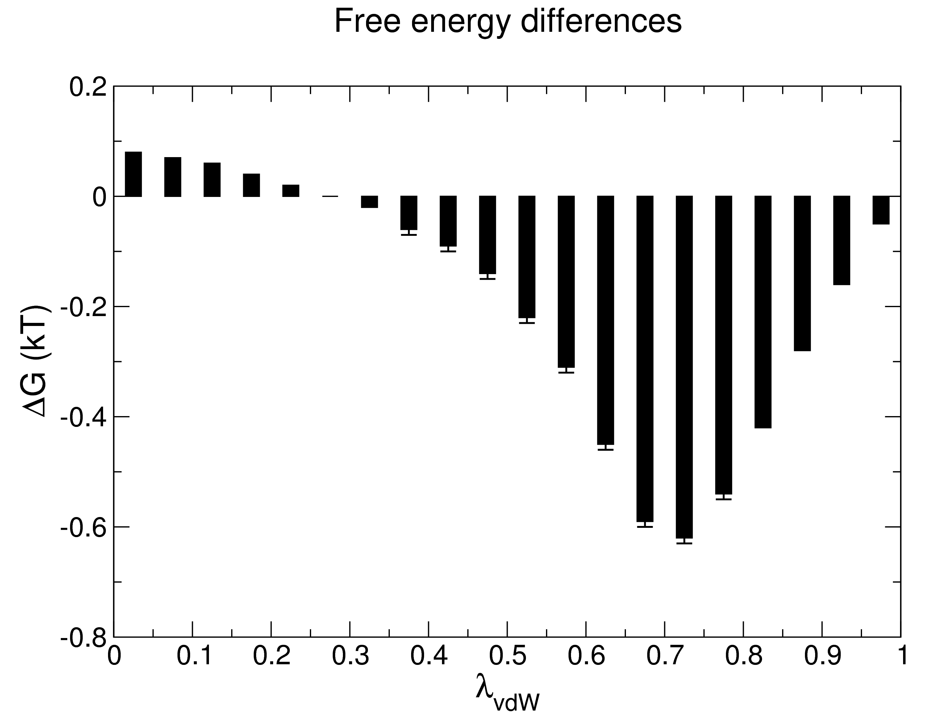
The bar module of GROMACS makes the calculation of ΔGAB very simple. Simply collect all of the md*.xvg files that were produced by mdrun (one for each value of λ) in the working directory and run gmx bar: GROMACS 的 bar 模块使ΔG AB 的计算非常简单。只需在工作目录中收集所有由 mdrun 生成的 md*.xvg 文件（每个λ值一个），然后运行 gmx bar： gmx bar -f md*.xvg -o -oi The program will print lots of useful information to the screen, in addition to producing three output files: bar.xvg, barint.xvg, and histogram.xvg. The screen output from gmx bar should look something like: 程序将在屏幕上打印大量有用信息，并生成三个输出文件：bar.xvg、barint.xvg 和 histogram.xvg。gmx bar 的屏幕输出应类似于： Detailed results in kT (see help for explanation): lam_A lam_B DG +/- s_A +/- s_B +/- stdev +/- 0 1 0.08 0.00 0.03 0.00 0.03 0.00 0.25 0.00 1 2 0.07 0.00 0.03 0.00 0.03 0.00 0.25 0.00 2 3 0.06 0.00 0.03 0.00 0.04 0.00 0.26 0.00 3 4 0.04 0.00 0.04 0.00 0.05 0.00 0.28 0.00 4 5 0.02 0.00 0.03 0.00 0.04 0.00 0.29 0.00 5 6 0.00 0.00 0.05 0.00 0.06 0.00 0.30 0.00 6 7 -0.02 0.00 0.05 0.00 0.06 0.00 0.32 0.00 7 8 -0.06 0.01 0.06 0.00 0.07 0.00 0.35 0.01 8 9 -0.09 0.01 0.06 0.00 0.07 0.00 0.37 0.00 9 10 -0.14 0.01 0.08 0.00 0.10 0.01 0.41 0.01 10 11 -0.22 0.01 0.09 0.01 0.12 0.01 0.46 0.00 11 12 -0.31 0.01 0.12 0.01 0.15 0.01 0.51 0.01 12 13 -0.45 0.01 0.17 0.01 0.20 0.01 0.57 0.00 13 14 -0.59 0.01 0.16 0.02 0.17 0.02 0.58 0.01 14 15 -0.62 0.01 0.11 0.01 0.11 0.01 0.47 0.00 15 16 -0.54 0.01 0.06 0.01 0.06 0.01 0.35 0.00 16 17 -0.42 0.00 0.03 0.01 0.03 0.01 0.25 0.00 17 18 -0.28 0.00 0.02 0.00 0.02 0.00 0.18 0.00 18 19 -0.16 0.00 0.01 0.00 0.01 0.00 0.13 0.00 19 20 -0.05 0.00 0.00 0.00 0.00 0.00 0.10 0.00 Final results in kJ/mol: point 0 - 1, DG 0.19 +/- 0.00 point 1 - 2, DG 0.17 +/- 0.01 point 2 - 3, DG 0.14 +/- 0.00 point 3 - 4, DG 0.09 +/- 0.01 point 4 - 5, DG 0.06 +/- 0.00 point 5 - 6, DG 0.01 +/- 0.01 point 6 - 7, DG -0.06 +/- 0.01 point 7 - 8, DG -0.14 +/- 0.02 point 8 - 9, DG -0.23 +/- 0.01 point 9 - 10, DG -0.35 +/- 0.01 point 10 - 11, DG -0.53 +/- 0.01 point 11 - 12, DG -0.77 +/- 0.03 point 12 - 13, DG -1.12 +/- 0.03 point 13 - 14, DG -1.46 +/- 0.02 point 14 - 15, DG -1.53 +/- 0.04 point 15 - 16, DG -1.35 +/- 0.02 point 16 - 17, DG -1.04 +/- 0.01 point 17 - 18, DG -0.70 +/- 0.01 point 18 - 19, DG -0.40 +/- 0.00 point 19 - 20, DG -0.13 +/- 0.00 total 0 - 20, DG -9.13 +/- 0.09 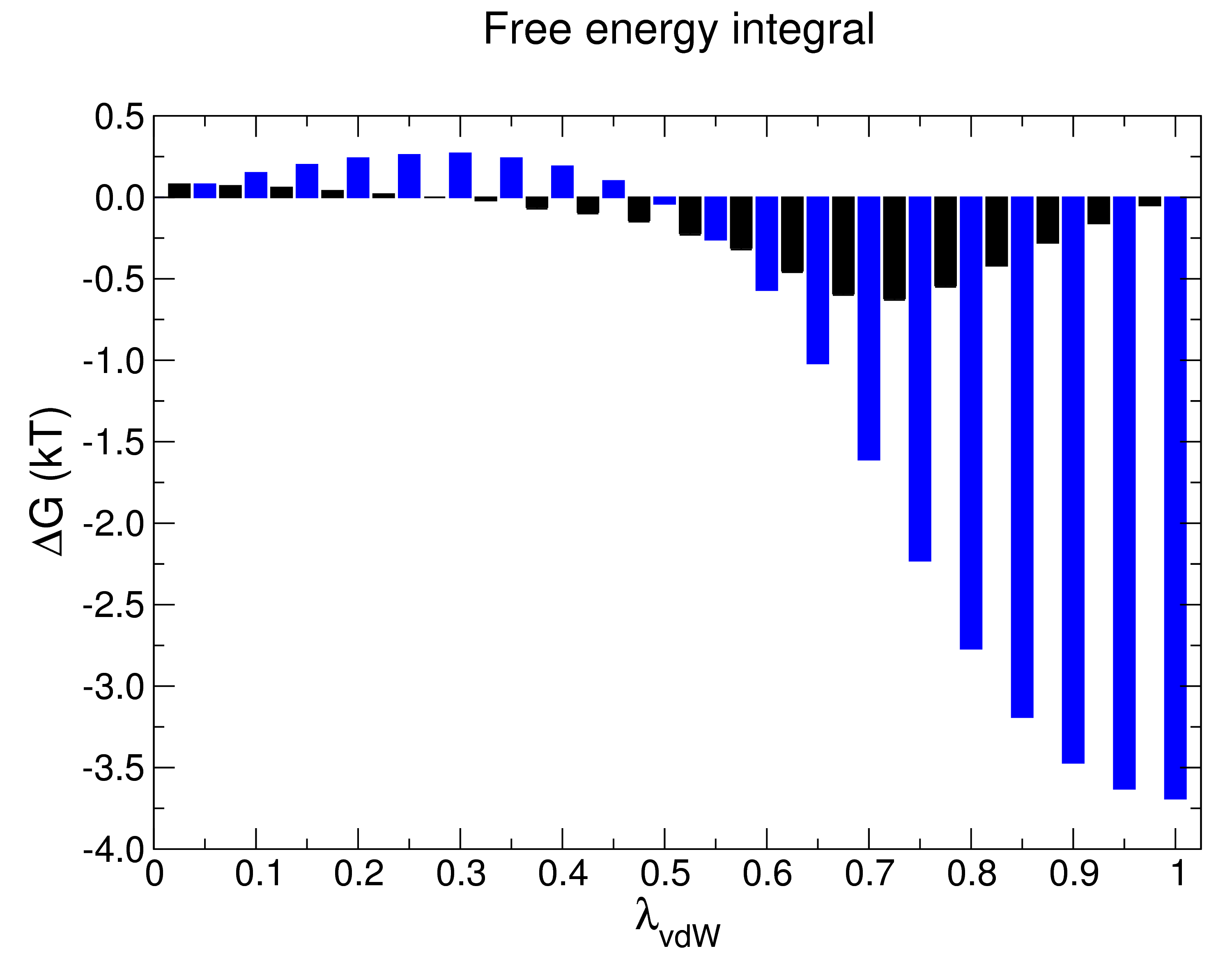The value of ΔGAB I obtained is -9.13 ± 0.09 kJ mol-1, or -2.18 ± 0.02 kcal mol-1. Since the process I conducted for this demonstration was the decoupling of methane, the reverse process (the introduction of uncharged methane into water, thus the actual hydration energy of the process) corresponds to a ΔGAB of 2.18 ± 0.02 kcal mol-1 (assuming reversibility), in good agreement with the value obtained by Shirts et al. of 2.24 ± 0.01 kcal mol-1 (per Table II of the Supporting Information of that paper), despite the fact that I used about half the number of λ vectors for the van der Waals transformation than the original authors did, in addition to the other changes described previously. 我获得的ΔG AB 值为-9.13 ± 0.09 kJ mol -1 ，或-2.18 ± 0.02 kcal mol -1 。由于本次演示进行的过程是甲烷解耦，其逆过程（将未带电的甲烷引入水中，即该过程的实际水合能）对应于ΔG AB 为 2.18 ± 0.02 kcal mol -1 （假设可逆性），与 Shirts 等人获得的结果 2.24 ± 0.01 kcal mol -1 （如表 II 的补充信息所示）吻合良好，尽管我在范德华变换中使用的λ向量数量约为原始作者的一半，并且还进行了其他先前描述的更改。 Technically, this is all we need to do to arrive at our answer, but gmx bar also prints a number of useful output files (all of which are optional). Their contents are worth exploring here, as they provide a great level of detail into the decoupling process and the success of sampling. 从技术上讲，这就是我们得出答案所需的所有步骤，但 gmx bar 还会打印一些有用的输出文件（所有这些文件都是可选的）。它们的內容值得在这里探讨，因为它们提供了关于解耦过程和采样成功程度的详细信息。   Output file 1: bar.xvg 输出文件 1：bar.xvg Let's take a look at the other output files that gmx bar gave us, starting with bar.xvg. This output file plots the relative free energy differences for each interval of λ (i.e., between neighboring Hamiltonians), and should look something like this (after re-plotting as a bar graph rather than the default line representation, and adding a few grid lines for perspective): 让我们看看 gmx bar 给出的其他输出文件，首先是 bar.xvg。这个输出文件绘制了每个λ间隔（即相邻哈密顿量之间）的相对自由能差异，看起来应该像这样（重新绘制为条形图而不是默认的线形表示，并添加几条网格线以供参考）： The vertical gray lines indicate the values of λ utilized in the decoupling process conducted here. Thus, each black bar indicates the free energy difference between neighboring values of λ. In bar.xvg, we get the first look at what calc_lambda_neighbors was doing during the simulations. For example, in our simulation of init_lambda_state = 0, the free energy at λ = 0.05 (the nearest neighboring window, as specified by calc_lambda_neighbors = 1) was evaluated every nstdhdl (10) steps. These "foreign" λ calculations result in energetic overlap between the values of λ, such that we have phase space overlap and adequate sampling. Interested readers should refer to the paper by Wu and Kofke cited in the gmx bar description for a discussion of this concept as well as the interpretation of the entropy values sA and sB. 垂直的灰线表示在此解耦过程中使用的λ值。因此，每个黑色条表示相邻λ值之间的自由能差。在 bar.xvg 中，我们首次看到了 calc_lambda_neighbors 在模拟过程中所做的工作。例如，在我们的 init_lambda_state = 0 模拟中，λ = 0.05（由 calc_lambda_neighbors = 1 指定的最近邻窗口）的自由能每隔 nstdhdl（10）步被评估一次。这些“外来”的λ计算导致λ值之间存在能量重叠，从而产生相空间重叠和充分的采样。感兴趣的读者应参考 gmx bar 描述中引用的 Wu 和 Kofke 的论文，以讨论这一概念以及熵值 s A 和 s B 的解释。 Thus, the free energy change from λ = 0 to λ = 1 is simply the sum of the free energy changes of each pair of neighboring λ simulations, which are plotted in bar.xvg. 因此，从λ = 0 到λ = 1 的自由能变化简单地是每个相邻λ模拟自由能变化的总和，这些变化在 bar.xvg 中绘制出来。 The values of ΔG correspond to the first half of the output printed to the screen by gmx bar. The second half of the screen output contains these same values of ΔG, converted to kJ mol-1 (1 kT = 2.478 kJ mol-1 at 298 K). ΔG 的值对应于 gmx bar 在屏幕上输出的前半部分。屏幕输出的后半部分包含这些相同的ΔG 值，已转换为 kJ mol -1 （在 298 K 时，1 kT = 2.478 kJ mol -1 ）。   Output file 2: barint.xvg 输出文件 2：barint.xvg The barint.xvg file plots the cumulative ΔG as a function of λ. In barint.xvg, the point at λ = 1 corresponds to the sum of ΔG from λ vector 0 to λ vector 1, as indicated in the screen output above: barint.xvg 文件绘制了累积ΔG 随λ的变化关系。在 barint.xvg 中，λ = 1 处的点对应于从λ向量 0 到λ向量 1 的ΔG 之和，如屏幕输出所示： lam_A lam_B DG +/- s_A +/- s_B +/- stdev +/- 0 1 0.08 0.00 0.03 0.00 0.03 0.00 0.25 0.00 1 2 0.07 0.00 0.03 0.00 0.03 0.00 0.25 0.00 Therefore, the value of the cumulative ΔG in barint.xvg at λ = 0 is zero, and the value at λ = 0.1 is 0.0 + 0.08 = 0.08, and this is the value we find in barint.xvg. Below is the plot of barint.xvg (blue) alongside the contents of bar.xvg (black, the values of ΔG between λ values) to illustrate the cumulative ΔG. By taking the value of ΔG at λ = 20 (-3.69 kT), we can recover the value of ΔG shown above (-9.14 kJ mol-1). The difference between the value here (-9.14) and above (-9.13) is due to rounding error from using only two decimal places, whereas the bar program is using full precision in its calculations above, but printing only two decimal places for all output. 因此，在 barint.xvg 中，λ = 0 处的累积ΔG 值为零，λ = 0.1 处的值为 0.0 + 0.08 = 0.08，这与我们在 barint.xvg 中观察到的一致。以下是 barint.xvg（蓝色）与 bar.xvg（黑色，λ值之间的ΔG 值）的对比图，以说明累积ΔG。通过取λ = 20 处的ΔG 值（-3.69 kT），我们可以恢复上述显示的ΔG 值（-9.14 kJ mol -1 ）。此处值（-9.14）与上述值（-9.13）之间的差异是由于仅使用两位小数导致的舍入误差，而 bar 程序在上述计算中使用了完整精度，但所有输出仅打印两位小数。

Advanced Applications  高级应用

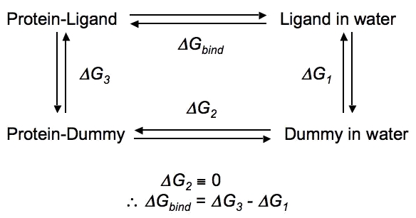
One common application of calculating free energies is to determine the of ΔG of binding between a ligand and a receptor (e.g., a protein), you would need to perform (de)coupling of the ligand in complex with the receptor and in bulk solution, since ΔG is (in this case) the sum of the free energy change of complexation of the ligand and receptor (i.e. the introduction of the ligand into the binding site) and the free energy of desolvating the ligand (i.e. removing it from solution): 计算自由能的一个常见应用是确定配体与受体（例如蛋白质）之间结合的ΔG 值。为此，你需要对与受体结合的配体以及在溶液中的配体进行（解）耦合，因为在这种情况下，ΔG 是配体与受体结合的自由能变化（即配体引入结合位点的自由能变化）与配体去溶剂化的自由能（即将其从溶液中移除）的总和： ΔGbind = ΔGcomplexation + ΔGdesolvation ΔGsolvation = -ΔGdesolvation ∴ ΔGbind = ΔGcomplexation - ΔGsolvation ΔG of binding will be the difference between these two states, and can be calculated through the use of the following (somewhat simplified) thermodynamic cycle, wherein ΔG1 is ΔGsolvation and ΔG3 is ΔGcomplexation in the equations above. 结合能的ΔG 将是这两个状态之间的差值，可以通过以下（简化版）的热力学循环计算，其中ΔG 1 是上述方程中的ΔG solvation ，ΔG 3 是ΔG complexation 。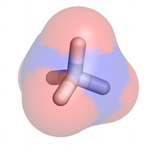 A particularly detailed thermodynamic cycle for this type of process can be found in Figure 1 of this paper. 这类过程的热力学循环可以特别详细地在本论文的图 1 中找到。 The transformation of a fully-interacting species (e.g., the ligand) into a "dummy" (a set of atomic centers in the configuration of the ligand that does not engage in any nonbonded interactions with its surroundings) requires turning off both van der Waals interactions (as demonstrated in this tutorial) and Coulombic interactions between the solute of interest and its surrounding environment. The complete series of transformations for methane is shown below: 将完全相互作用的物种（例如配体）转化为“虚拟”（在配体构型中不与其周围环境发生任何非键相互作用的一组原子中心）需要关闭范德华相互作用（如本教程所示）以及目标溶质与其周围环境之间的库仑相互作用。甲烷的完整转化系列如下所示： Fully-interacting  完全相互作用 No charges, full LJ 无电荷，完整 LJ Dummy molecule  虚拟分子 In the above thermodynamic cycle, ΔG1 and ΔG3 actually represent the introduction of the ligand (starting as a dummy molecule), i.e. coupling rather than decoupling. The thermodynamic cycle above is extremely basic, and does not account for considerations like orientational restraints, conformational changes of the protein, etc. None of this literature will be discussed here. For most small molecules (generically named "LIG" below), the following settings might seem attractive: 在上述热力学循环中，ΔG 1 和 ΔG 3 实际上代表配体的引入（最初作为虚拟分子），即耦合而非解耦。上述热力学循环非常基础，没有考虑诸如方向约束、蛋白质构象变化等。这里不会讨论这些文献。对于大多数小分子（以下统称为"LIG"），以下设置可能看起来很有吸引力： couple-moltype = LIG couple-intramol = no couple-lambda0 = none couple-lambda1 = vdw-q Special care must be taken in this case. In previous versions of GROMACS, such an approach was likely to be very unstable because removal of van der Waals terms while a system retains some charge allows oppositely-charged atoms to interact very closely (in the absence of the full effects of an electron cloud). The result would be unstable configurations and unreliable energies, even if the systems didn't collapse. Thus, it is more sound to approach the (de)coupling sequentially. In version 5.0, this is very easily done with the new λ vector capabilities: 在这种情况下必须特别小心。在 GROMACS 的早期版本中，这种方法很可能非常不稳定，因为在系统保留部分电荷的同时移除范德华项，会导致异种电荷的原子非常接近（在没有电子云的完整效应的情况下）。即使系统没有崩溃，结果也会是不稳定的构型和不可靠的能量。因此，按顺序进行（解）耦合更为稳妥。在 5.0 版本中，利用新的λ向量功能可以非常容易地完成这一点： couple-moltype = LIG couple-intramol = no couple-lambda0 = none couple-lambda1 = vdw-q init_lambda_state = 0 calc_lambda_neighbors = 1 vdw_lambdas = 0.00 0.05 0.10 ... 1.00 1.00 1.00 ... 1.00 coul_lambdas = 0.00 0.00 0.00 ... 0.00 0.05 0.10 ... 1.00 In this case, the λ value for Coulombic interactions is always zero while the λ value for transforming van der Waals interactions changes. Then, the van der Waals interactions are fully on (λ = 1.00) while the Coulombic interactions are gradually turned on. Keeping track of the states to which λ = 0 and λ = 1 correspond is key to this process. In the above case, couple-lambda0 says interactions are off, while couple-lambda1 means interactions are on. 在这种情况下，库仑相互作用的λ值始终为零，而用于转换范德华相互作用的λ值会变化。然后，范德华相互作用完全开启（λ = 1.00），而库仑相互作用逐渐开启。了解λ = 0 和λ = 1 分别对应的状态是此过程的关键。在上述情况下，couple-lambda0 表示相互作用关闭，而 couple-lambda1 表示相互作用开启。 These types of transformations can be useful for calculating hydration/solvation free energies, since this quantity is often used as target data in force field parametrization. 这类转换对于计算水合/溶剂化自由能很有用，因为该量通常用作力场参数化的目标数据。

Summary  摘要

You have now calculated the free energy change for a simple transformation that has previously been calculated with high precision, the decoupling of van der Waals interactions between a simple solute (uncharged methane) and solvent (water). Hopefully this tutorial will provide you with the understanding necessary to take on more complex systems. 您现在已经计算了一个简单转变的自由能变化，这个转变之前已经被以很高的精度计算过，即一个简单溶质（不带电的甲烷）和溶剂（水）之间的范德华相互作用的解耦。希望这个教程能为您提供必要的理解，以便您能够处理更复杂的系统。 If you have suggestions for improving this tutorial, if you notice a mistake, or if anything is otherwise unclear, please feel free to email me. Please note: this is not an invitation to email me for GROMACS problems. I do not advertise myself as a private tutor or personal help service. That's what the GROMACS User Forum is for. I may help you there, but only in the context of providing service to the community as a whole, not just the end user. 如果您对本教程有任何改进建议，如果您发现错误，或者如果任何内容仍不清晰，请随时通过电子邮件与我联系。请注意：这不是邀请我通过电子邮件解决 GROMACS 问题。我不将自己宣传为私人导师或个人帮助服务。GROMACS 用户论坛才是为此目的。我可能会在那里提供帮助，但仅限于为整个社区提供服务，而不仅仅是最终用户。 Happy simulating!  模拟愉快！