机器学习基础算法11-Logistic回归-ROC和AUC分类模型评估-实例

一、模型评估介绍

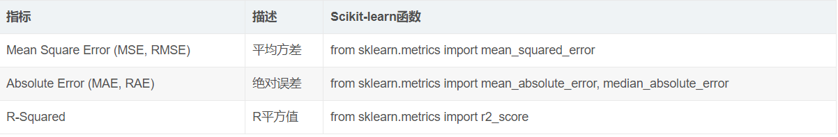
1.分类模型评估

2.回归模型评估

二、ROC和AUC

1.理论知识

AUC概念理解： https://www.zhihu.com/question/39840928?from=profile_question_card

ROC全称是“受试者工作特征”（Receiver Operating Characteristic）。ROC曲线的面积就是AUC（Area Under the Curve）。AUC用于衡量“二分类问题”机器学习算法性能（泛化能力）。

ROC曲线是二值分类问题的一个评价指标。它是一个概率曲线，在不同的阈值下绘制TPR与FPR的关系图，从本质上把“信号”与“噪声”分开。

AUC越大表明当前分类算法分类效果越好

截断点（阈值）取不同的值，TPR和FPR的计算结果也不同。将截断点不同取值下对应的TPR和FPR结果画于二维坐标系中得到的曲线，就是ROC曲线。横轴用FPR表示。

2. ROC曲线分析

random chance这条直线是随机概率，一半的概率是对的，一半的概率是错的。如果低于这条线，说明算法极差，都不如随机猜的。因此在这条线的左边说明算法还好点。

3.TPR与FPR的计算过程

y = [0,0,1,1]
y_pre = [0.1,0.5,0.3,0.8]
阈值分别取：0.1,0.3,0.5,1

阈值为0.1时

y1=[1,1,1,1]

阈值为0.3时

y2=[0,1,1,1]

阈值为0.5时

y3 = [0,1,0,1]

阈值为0.8时

y4 = [0,0,0,1]

三、实例

1.实例1

sklearn.metrics.roc_curve介绍： https://blog.csdn.net/sun91019718/article/details/101314545

# AUC举例-画出ROC曲线
import numpy as np
# 模型评估
from sklearn import metrics
import matplotlib as mpl
import matplotlib.pyplot as plt


if __name__ == '__main__':
    y = np.array([0, 0, 1, 1])
    y_pred = np.array([0.1, 0.5, 0.3, 0.8])

    # 返回三个数组结果分别是fpr(假正率),tpr(召回率),threshold(阈值)
    # 参数为真实结果数据、预测结果数据（可以是标签数据也可以是概率值）
    fpr,tpr,threshold = metrics.roc_curve(y,y_pred)
    # # np.insert将向量插入某一行或列
    # fpr = np.insert(fpr, 0, 0)
    # tpr = np.insert(tpr, 0, 0)
    print(fpr)
    print(tpr)
    print(threshold)
    # 计算AUC的值
    auc = metrics.auc(fpr, tpr)
    print(metrics.roc_auc_score(y, y_pred))

    # 解决matplotlib 中不能识别中文的问题
    mpl.rcParams['font.sans-serif'] = u'SimHei'
    mpl.rcParams['axes.unicode_minus'] = False

    plt.figure(figsize=(10,10), facecolor='w')
    # markerfacecolor =mfc linewidth=lw linestyle=ls  markeredgecolor = mec
    plt.plot(fpr, tpr, marker='o', lw=5, ls='-', mfc='g', mec='g', color='r')
    plt.plot([0, 1], [0, 1], lw=5, ls='--', c='b')

    # 调整坐标轴范围
    plt.xlim((-0.01, 1.02))
    plt.ylim((-0.01, 1.02))

    # 设置x轴、y轴的刻度
    plt.xticks(np.arange(0, 1.1, 0.1))
    plt.yticks(np.arange(0, 1.1, 0.1))

    # 设置行标签与列标签
    plt.xlabel('False Positive Rate', fontsize=20)
    plt.ylabel('True Positive Rate', fontsize=20)

    # 设置网格线
    plt.grid(b=True, ls='dotted')

    # 设置标题
    plt.title(u'ROC曲线', fontsize=20)
    plt.show()

[0.  0.  0.5 0.5 1. ]
[0.  0.5 0.5 1.  1. ]
[1.8 0.8 0.5 0.3 0.1]
0.75