路透社新闻分类（多分类）--python深度学习

import keras
keras.__version__

‘2.0.8’

路透社新闻分类（多分类）

多分类任务（Keras内置数据集）

路透社数据集，它包含许多短新闻及其对应的主题，由路透社在 1986 年发布。它是一个简单的、广泛使用的文本分类数据集。

• 包括 46 个不同的主题

1.数据导入

from keras.datasets import reuters

(train_data, train_labels), (test_data, test_labels) = reuters.load_data(num_words=10000)

IMDB 数据集一样，参数 num_words=10000 将数据限定为前 10 000 个最常出现的单词

len(train_data)

8982

len(test_data)

2246

# 与 IMDB 评论一样，每个样本都是一个整数列表（表示单词索引）
train_data[10]

# 样本对应的标签是一个 0~45 范围内的整数
train_labels[10]

3

将索引解码为新闻文本：索引减去了 3，因为 0、1、2 是为“padding”（填充）、“start of
sequence”（序列开始）、“unknown”（未知词）分别保留的索引

word_index = reuters.get_word_index()
reverse_word_index = dict([(value, key) for (key, value) in word_index.items()])
decoded_newswire = ' '.join([reverse_word_index.get(i - 3, '?') for i in train_data[0]])

decoded_newswire

‘? ? ? said as a result of its december acquisition of space co it expects earnings per share in 1987 of 1 15 to 1 30 dlrs per share up from 70 cts in 1986 the company said pretax net should rise to nine to 10 mln dlrs from six mln dlrs in 1986 and rental operation revenues to 19 to 22 mln dlrs from 12 5 mln dlrs it said cash flow per share this year should be 2 50 to three dlrs reuter 3’

2.数据预处理

# seasons = ['Spring', 'Summer', 'Fall', 'Winter']
# list(enumerate(seasons))

[(0, ‘Spring’), (1, ‘Summer’), (2, ‘Fall’), (3, ‘Winter’)]

(1)数据向量化(One-hot编码)

import numpy as np

def vectorize_sequences(sequences, dimension=10000):
    results = np.zeros((len(sequences), dimension))
    for i, sequence in enumerate(sequences):
        results[i, sequence] = 1.
    return results

# 训练数据向量化
x_train = vectorize_sequences(train_data)
# 测试数据向量化
x_test = vectorize_sequences(test_data)

array([[0., 1., 0., …, 0., 0., 0.],
[0., 0., 0., …, 0., 0., 0.],
[0., 0., 0., …, 0., 0., 0.]])

(2)标签向量化(One-hot编码)

# 方法一：自定义函数
def to_one_hot(labels, dimension=46):
    results = np.zeros((len(labels), dimension))
    for i, label in enumerate(labels):
        results[i, label] = 1.
    return results

# 训练标签
one_hot_train_labels = to_one_hot(train_labels)
# 测试标签
one_hot_test_labels = to_one_hot(test_labels)

# 方法二：Keras 内置方法
from keras.utils.np_utils import to_categorical

one_hot_train_labels = to_categorical(train_labels)
one_hot_test_labels = to_categorical(test_labels)

3. 模型构建

对于前面用过的 Dense的堆叠，每层只能访问上一层输出的信息。如果某一层丢失了与
分类问题相关的一些信息，那么这些信息无法被后面的层找回，每一层都可能成为
信息瓶颈。

16 维空间可能太小了，无法学会区分 46 个不同的类别，故设置64 个单元。

# 1.模型定义
from keras import models
from keras import layers

model = models.Sequential()
model.add(layers.Dense(64, activation='relu', input_shape=(10000,)))
model.add(layers.Dense(64, activation='relu'))
model.add(layers.Dense(46, activation='softmax'))

# 2.模型编译
model.compile(optimizer='rmsprop',
              loss='categorical_c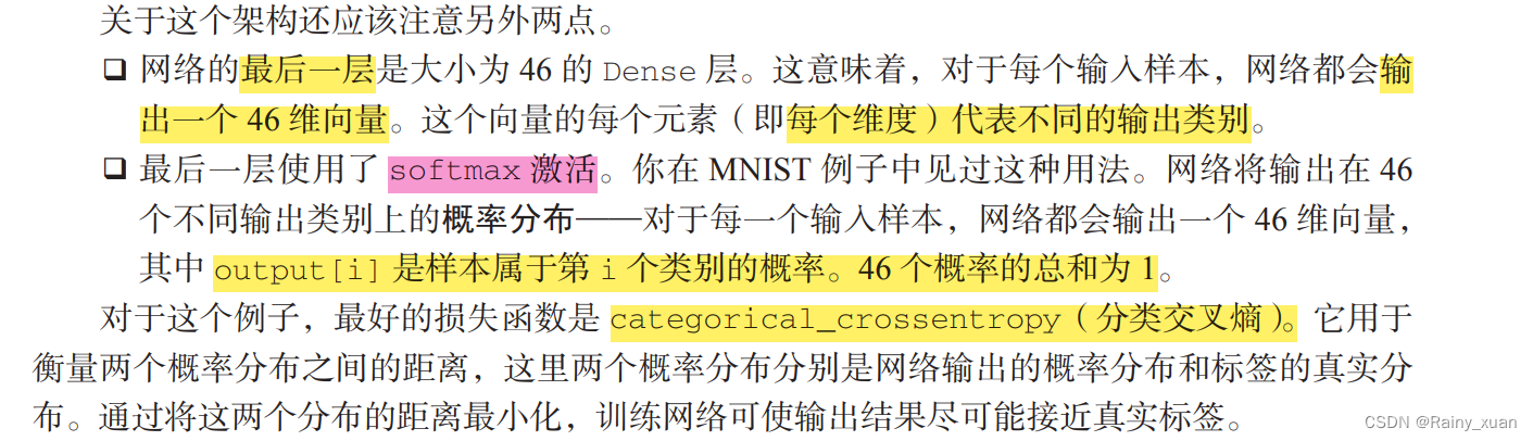![在这里插入图片描述](https://img-blog.csdnimg.cn/649dd0dcc3e74f76b4cbefbac741b99d.png)
rossentropy',   # 分类交叉熵
              metrics=['accuracy'])

4. 验证

在训练数据中留出 1000 个样本作为验证集

x_val = x_train[:1000]
partial_x_train = x_train[1000:]

y_val = one_hot_train_labels[:1000]
partial_y_train = one_hot_train_labels[1000:]

# 3.模型训练(fit)
history = model.fit(partial_x_train,
                    partial_y_train,
                    epochs=20,
                    batch_size=512,
                    validation_data=(x_val, y_val))

history_dict = history.history
history_dict.keys()

dict_keys([‘loss’, ‘accuracy’, ‘val_loss’, ‘val_accuracy’])

绘制损失曲线和精度曲线

import matplotlib.pyplot as plt

loss = history.history['loss']
val_loss = history.history['val_loss']

epochs = range(1, len(loss) + 1)

plt.plot(epochs, loss, 'bo', label='Training loss')    # 'bo' 表示蓝色圆点
plt.plot(epochs, val_loss, 'b', label='Validation loss')    # 'b' 表示蓝色实线
plt.title('Training and validation loss')
plt.xlabel('Epochs')
plt.ylabel('Loss')
plt.legend()

plt.show()

plt.clf()   # clear figure

acc = history.history['accuracy']
val_acc = history.history['val_accuracy']

plt.plot(epochs, acc, 'bo', label='Training acc')
plt.plot(epochs, val_acc, 'b', label='Validation acc')
plt.title('Training and validation accuracy')
plt.xlabel('Epochs')
plt.ylabel('Loss')
plt.legend()

plt.show()

网络在训练 9 轮后开始过拟合,重新训练网络

model = models.Sequential()
model.add(layers.Dense(64, activation='relu', input_shape=(10000,)))
model.add(layers.Dense(64, activation='relu'))
model.add(layers.Dense(46, activation='softmax'))

model.compile(optimizer='rmsprop',
              loss='categorical_crossentropy',
              metrics=['accuracy'])
model.fit(partial_x_train,
          partial_y_train,
          epochs=8,
          batch_size=512,
          validation_data=(x_val, y_val))
results = model.evaluate(x_test, one_hot_test_labels)

results

[0.9732478260993958, 0.7867319583892822]

如果是一个完全随机的分类器哈哈哈

import copy

test_labels_copy = copy.copy(test_labels)
np.random.shuffle(test_labels_copy)
float(np.sum(np.array(test_labels) == np.array(test_labels_copy))) / len(test_labels)

0.18477292965271594

5.预测

predictions = model.predict(x_test)

# predictions 中的每个元素都是长度为 46 的向量
predictions.shape

(2246, 46)

# 每个元素的总和为 1
np.sum(predictions[0])

0.99999994

np.argmax()：获取array的某一个维度中数值最大的那个元素的索引

# 概率最大的类别就是预测类别
np.argmax(predictions[0])

3

番外1：处理label和loss的其他方法

之前采用One-hot编码，现在采用第一种：转化为整数张量

y_train = np.array(train_labels)
y_test = np.array(test_labels)

改变损失函数的选择：

• 分类（One-hot）编码：使用categorical_crossentropy
• 整数标签：使用sparse_categorical_crossentropy

model.compile(optimizer='rmsprop', loss='sparse_categorical_crossentropy', metrics=['acc'])

新的损失函数在数学上与 categorical_crossentropy 完全相同，二者只是接口不同

番外2： 中间层维度足够大的重要性

model = models.Sequential()
model.add(layers.Dense(64, activation='relu', input_shape=(10000,)))
model.add(layers.Dense(4, activation='relu'))
model.add(layers.Dense(46, activation='softmax'))

model.compile(optimizer='rmsprop',
              loss='categorical_crossentropy',
              metrics=['accuracy'])
model.fit(partial_x_train,
          partial_y_train,
          epochs=20,
          batch_size=128,
          validation_data=(x_val, y_val))

现在网络的验证精度最大约为 71%，比前面下降了 8%。导致这一下降的主要原因在于，试图将大量信息（这些信息足够恢复 46 个类别的分割超平面）压缩到维度很小的中间空间。网络能够将大部分必要信息塞入这个四维表示中，但并不是全部信息。