使用聚类模型|客户对汽车满意度数据集聚类

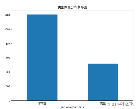
        数据集从汽车的价格、质量、及舒适度这三个方面的相关数据出发，对汽车的客户满意度进行分类预测。数据一共包含6个相关特征，1个类别变量（即汽车满意度），共1728个样本点。

	buying	maint	doors	persons	lug_boot	safety
count	1728	1728	1728	1728	1728	1728
mean	2.5	2.5	2.5	2	2	2
std	1.1183576	1.11835	1.1183576	0.816732	0.816732	0.81673
min	1	1	1	1	1	1
25%	1.75	1.75	1.75	1	1	1
50%	2.5	2.5	2.5	2	2	2
75%	3.25	3.25	3.25	3	3	3
max	4	4	4	3	3	3

原样本中的标签数量。聚类前，先把标签都删除。

        “物以类聚，人以群分”，将数据集中相似的样本分到一组，每个组称为一个簇(cluster)，相同簇的样本之间相似度较高，不同簇的样本之间相似度较低。样本之间的相似度通常是通过距离定义的，距离越远，相似度越低。

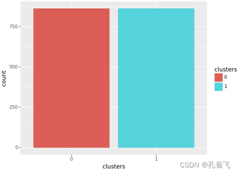
        本文主要采用K-Means算法和Meanshift算法对数据进行聚类分析。当使用K-Means模型时，聚类值取2类，得到的直方图。此时，模型的轮廓系数为0.1664。当Cluster取不同的值时，得到轮廓系数折线图。

        当使用Meanshift算法采用不同窗宽时，其对应的轮廓系数如图所示，当窗宽为2时，轮廓系数达到最大，且此时的簇的个数为2。具体数值如表所示。 

	Bandwidth	Cluster_number	Silhouette_score
0	1.0	362	0.0411
1	1.2	864	-0.0141
2	1.4	48	0.1262
3	1.6	16	0.1354
4	1.8	8	0.1325
5	2.0	2	0.1424

Kmeans代码如下：

import warnings
warnings.filterwarnings("ignore")
import numpy as np
import pandas as pd
from plotnine import *
from sklearn import metrics
from sklearn.cluster import KMeans
import matplotlib.pyplot as plt

# 读入数据
auto = pd.read_csv('Car.csv')

plt.rcParams['font.sans-serif'] = ['SimHei']

plt.figure(figsize=(8, 6))
auto.car_acceptability.value_counts().plot(kind='bar', rot=360, title='类别数量分布条形图')
plt.xticks([1, 0], ['满意', '不满意'])
plt.show()
model = KMeans(n_clusters=2,random_state=111).fit(auto)    #为使复现效果与PPT效果相同，设置随机种子为111
#样本标签和簇质心
auto_label = model.labels_
auto_cluster = model.cluster_centers_
auto_label

#画每个簇样本数的柱状图
auto_label_dataframe = pd.DataFrame({'clusters':auto_label})
auto_label_dataframe['clusters'] = auto_label_dataframe['clusters'].astype('category')
a=ggplot(auto_label_dataframe,aes('clusters',fill='clusters')) + geom_bar()
#print(a)

# 轮廓系数评估聚类效果
labels = model.labels_
print("轮廓系数(Silhouette Coefficient): %0.4f"
      % metrics.silhouette_score(auto, labels))
label=[]
k=np.arange(2,7,1)
for i in k:
    model = KMeans(n_clusters=i,random_state=111).fit(auto)  
    labels = model.labels_
    label.append(round(metrics.silhouette_score(auto, model.labels_), 4))
plt.plot(k,label, marker='.', linestyle='-', color='g')
plt.title('Silhouette Coefficient vs Number of Clusters')
plt.xlabel('Number of Clusters')
plt.ylabel('Silhouette Coefficient')
#plt.legend()
#plt.show()

Meanshift代码如下：

# 读入数据
auto = pd.read_csv('Car.csv')
a=auto.describe()
print(a)
bandwidth_grid = np.arange(1, 2.1, 0.2)
cluster_number = []
slt_score = []
# 训练模型
for i in bandwidth_grid:
    model = MeanShift(bandwidth=i).fit(auto)
    cluster_number.append(len(np.unique(model.labels_)))
    slt_score.append(round(metrics.silhouette_score(auto, model.labels_), 4))
result = pd.DataFrame([])

result['bandwidth'] = bandwidth_grid
result['cluster_number'] = cluster_number
result['silhouette_score'] = slt_score

print(result)
# 得到标签和聚类中心
auto_label = model.labels_
auto_cluster = model.cluster_centers_
# 轮廓系数
labels = model.labels_
#找出簇质心连续性变量的坐标
centroid_cluster = pd.DataFrame(auto_cluster).copy().iloc[:,:6]
centroid_cluster.columns=['buying','maint','doors','persons','lug_boot','safety']
#将数据逆标准化，转换为原始数据
c=centroid_cluster.applymap(lambda x:'%.2f'%x)
print(c)
print("轮廓系数(Silhouette Coefficient): %0.4f"
      % metrics.silhouette_score(auto, labels))

plt.plot(bandwidth_grid,slt_score, marker='.', linestyle='-', color='g')
plt.title('Meanshift Clustering-Silhouette Score')
plt.xlabel('Bandwiths')
plt.ylabel('Silhouette Score')
#plt.legend()
plt.show()