基于Matlab的航向角导航

 

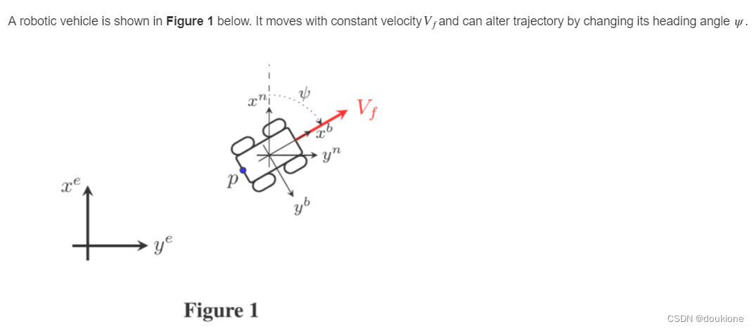
Using the nomenclature presented in your Navigation Systems course (mathematics section), the vehicle body frame () is the object frame while the reference frame () is defined at some fixed point on the earth's surface as shown. The position of the vehicle is then denoted , where γ can be either  or b. In this scenario, the vehicle velocity (), defined with respect to the body axes, yields an expression for the velocity observed in the object frame as,

By computing the appropriate velocity and acceleration vectors, write a MATLAB script that will track the position of the vehicle, resolved in earth axes, with the following control inputs:

assuming constant acceleration over each timestep, plot the resulting trajectory over 120s (2min). Use the integration schemes defined in the course notes to solve the ODE's for   and , i.e. trapezoidal integration and the fourth-order scheme for .

以下是Matlab代码：

%% Define simulation parameters
dt = 0.01;             % Simulation timestep (s)
t = 0:dt:120;           % Simulation time points
om = 0.2;               % Heading modulation frequency (rad/s)
V = 1.5;                % Vehicle velocity
k = 0.05;               % Heading modulation amplitude (rad)
om_ie_z = 7.292115e-5;    % Earth spin rate (rad/s)
om_ie = [0;0;om_ie_z];
Om_ie = [0 -om_ie_z 0;om_ie_z 0 0;0 0 0];
%% Initialise variables
r_eb_e = zeros(3,length(t));  % Start at the origin 
v_eb_e = zeros(3,length(t));  % Pre-allocate memory
vd_eb_e = zeros(3,length(t)); % Pre-allocate memory
om_ib_b_measured = zeros(3,length(t));  % Pre-allocate memory
f_ib_b_measured = zeros(3,length(t));   % Pre-allocate memory
psi0 = -0.24;                           % Initial vehicle Heading (rad)
Cbe = [cos(psi0) sin(psi0) 0;-sin(psi0) cos(psi0) 0;0 0 1]';           
                        % Body-to-Earth co-ord transformation matrix
Cbe_est = Cbe;          % Body-to-Earth co-ord transformation matrix (estimate)
u = [V;0;0];            % Absolute velocity resolved in body axes
v_eb_e(:,1) = Cbe*u;    % Initialise estimated velocity

%% Calculate the true trajectory
% In this section, the true vehicle trajectory will be calculated using a
% fourth-order numerical integration scheme. Therefore, the true vehicle
% trajectory will be contained in the 'y' matrix. 
%
y0 = [0;0;V*cos(psi0);V*sin(psi0);V;psi0;k*sin(psi0)];
[tx,y] = ode45(@(t,y)calcDerivatives(t,y,k,om,psi0),t,y0);

%% Define the error terms
errSwitch = 0;                  % Set this value to '1' to add constant errors and '0' otherwise
noiseSwitch = 0;                % Set this value to '1' to add noise and '0' otherwise
noisea = 0.0001*noiseSwitch*rand(3,length(t));    % Accelerometer white noise 
noiseg = 0.00001*noiseSwitch*rand(3,length(t));   % Gyro white noise 
ba = 1e-4*[1;1;1]*errSwitch;    % Accelerometer bias
sa = 1e-4*diag([1;1;1]);        % Accelerometer scale factor error
ma = [0 -0.0001 0.0003;0.0001 0 0.0002;-0.0001 -0.0002 0]; % Acc. cross coupling error
Ma = (sa + ma)*errSwitch;       % Combined accelerometer scale factor & cross coupling error matrix
bg = 1e-5*[1;1;1]*errSwitch;    % Gyro bias
sg = 1e-5*diag([1;1;1]);        % Gyro scale factor error
mg = [0 -0.0001 0.0003;0.0001 0 0.0002;-0.0001 -0.0002 0]; % Gyro cross coupling error
Mg = (sg + mg)*errSwitch;       % Combined gyro scale factor & cross coupling error matrix

%% Loop over time
for i=2:length(t)                  
    %
    % ***********************************************
    % *  Calculate the estimated INU trajectory     *
    % ***********************************************
    %
    % First step, we need to calculate the true values of specific force
    % and angular rate. These will be used to generate our simulated
    % measurements.
    % First, find the true angular rate
    psi = psi0 + om*t(i);
    om_ib_b_True = [0;0;k*sin(psi)] + Cbe_est*om_ie;
    Om_ib_b_True = [0 -om_ib_b_True(3,1) 0;...
                 om_ib_b_True(3,1) 0 0;0 0 0];
    % Next, calculate the true specific force
    f_ib_b_True = (Om_ib_b_True + Cbe_est'*Om_ie*Cbe_est)*u;
    
    
    % Add the errors onto the true angular rate and specific force vectors
    % to create the measurements. (Hint: add the gyro random noise term
    % using the following notation - noiseg(:,i). Sim for accelerometer
    % noise). First, the gyro measurement
    I=eye(3);
    om_ib_b_measured(:,i) = bg+(I+Mg)*om_ib_b_True+noiseg(:,i);
    Om_ib_b_measured = [0 -om_ib_b_measured(3,1) 0;...
        om_ib_b_measured(3,1) 0 0;0 0 0];      % Skew-symmetric matrix form
    % Now the accelerometer measurement
    f_ib_b_measured(:,i) = ba+(I+Ma)*f_ib_b_True+noisea(:,i);
                           
    % Although not explicitly required for this formulation, calculate the
    % strapdown equation in here i.e. find Cbd_dot_est.
    Cbe_dot_est = Cbe_est*Om_ib_b_True-(Om_ie*Cbe);
    
    % Navigation Equation goes in here
    vd_eb_e(:,i) = Cbe*f_ib_b_measured(:,i)-2*Om_ie*v_eb_e(:,(i-1));
                       
    % Now integrate all equations using the techniques present in the
    % notes i.e. fourth-order scheme for Cbe_est and trapezoidal
    % integration for acceleration and velocity
    % First, the DCM using the 4th order scheme. (Hint: when calculating
    % alpha, remember to use om_eb_b_measured).
    alpha = (om_ib_b_measured(:,i)-om_ie)*dt;
    alpha_norm = norm(alpha);
    if(alpha_norm > 0) % only update if there has been a rotation
    skew_alpha = [0 alpha(3,1) 0;...
        alpha(3,1) 0 0;0 0 0];            % Skew-symmetric matrix form
    Cbe_est = Cbe;
    end
    
    % Finally, integrate the velocity and position ODE's using the
    % trapezoidal rule. First, calculate the new velocity estimate,
    v_eb_e(:,i) = v_eb_e(:,(i-1))+((vd_eb_e(:,i)+vd_eb_e(:,(i-1)))/2)*dt ;
    % and the position estimate,
    r_eb_e(:,i) = r_eb_e(:,(i-1))+((v_eb_e(:,i)+v_eb_e(:,(i-1)))/2)*dt;
    
 
    
    % The following lines of code are used to store data for use in the assessments below.
    if(i==2)
        om_ib_b_check = om_ib_b_measured(:,i);
        f_ib_b_check = f_ib_b_measured(:,i);
        Cbe_dot_check = Cbe_dot_est;
        vd_eb_e_check = vd_eb_e(:,i);
        alpha_check = alpha;
        Cbe_check = Cbe_est;
        v_eb_e_check = v_eb_e(:,i);
        r_eb_e_check = r_eb_e(:,i);
    end
end
%
% Plot the results
figure(1);
% Plot the track
plot3(y(:,1),y(:,2),zeros(1,length(tx)),'b');
hold on;
plot3(r_eb_e(1,:),r_eb_e(2,:),-r_eb_e(3,:),'g'); 
xlabel('x (m)');
ylabel('y (m)');
zlabel('z (m)');
title('Vehicle trajectory');
legend('true','estimated','Location','NorthWest');
hold off;
% axis equal;
view(2);
grid on;
% Plot the error magnitude
figure(2);
plot(t,y(:,1)-r_eb_e(1,:)');
hold on;
plot(t,y(:,2)-r_eb_e(2,:)');
hold off;
xlabel('t (s)');
ylabel('error (m)');
title('Navigation errors vs. time');
legend('x-error','y-error','Location','SouthWest');
grid on;
%
figure(3);
plot(t,om_ib_b_measured(1:3,:));
xlabel('t(s)');
ylabel('\omega_i_b^b (rad/s)');
title(' Measured Angular rates \omega_i_b^b');
legend('p','q','r','Location','NorthWest');
grid on;
figure(4);
plot(t,f_ib_b_measured(1:2,:));
xlabel('t(s)');
ylabel('f_i_b^b (m/s^2)');
title('measured Specific force f_i_b^b');
legend('x-axis','y-axis','Location','SouthWest');
grid on;

function yd = calcDerivatives(t,y,k,beta,psi0)
%
yd = y;
yd(1,1) = y(5,1)*cos(y(6,1));           % xdot
yd(2,1) = y(5,1)*sin(y(6,1));           % ydot
yd(3,1) = -y(5,1)*sin(y(6,1))*y(7,1);   % xddot
yd(4,1) = y(5,1)*cos(y(6,1))*y(7,1);    % yddot
yd(5,1) = 0;                            % Vdot
yd(6,1) = k*sin(beta*t+psi0);           % psidot
yd(7,1) = k*beta*cos(beta*t+psi0);      % psiddot
end

其中的errSwitch和noiseSwitch可以设置为1，请尝试当errSwitch=1以及errSwitch和noiseSwitch都为1时图像的变化。