NNDL 作业8：RNN - 简单循环网络

最新推荐文章于 2023-07-06 15:09:21 发布

weixin_51715088

最新推荐文章于 2023-07-06 15:09:21 发布

阅读量103

点赞数 1

文章标签： rnn numpy python

本文链接：https://blog.csdn.net/weixin_51715088/article/details/127831310

版权

一、使用Numpy实现SRN

# coding=gbk
 
import numpy as np
 
inputs = np.array([[1., 1.],
                   [1., 1.],
                   [2., 2.]])  # 初始化输入序列
print('inputs is ', inputs)
 
state_t = np.zeros(2, )  # 初始化存储器
print('state_t is ', state_t)
 
w1, w2, w3, w4, w5, w6, w7, w8 = 1., 1., 1., 1., 1., 1., 1., 1.
U1, U2, U3, U4 = 1., 1., 1., 1.
print('--------------------------------------')
for input_t in inputs:
    print('inputs is ', input_t)
    print('state_t is ', state_t)
    in_h1 = np.dot([w1, w3], input_t) + np.dot([U2, U4], state_t)
    in_h2 = np.dot([w2, w4], input_t) + np.dot([U1, U3], state_t)
    state_t = in_h1, in_h2
    print('a',state_t,in_h1,in_h2)
    output_y1 = np.dot([w5, w7], [in_h1, in_h2])
    output_y2 = np.dot([w6, w8], [in_h1, in_h2])
    print('output_y is ', output_y1, output_y2)
    print('---------------')

输出结果：

E:\Python\python.exe "E:/pythonProject/ceshi 2.py"
inputs is  [[1. 1.]
 [1. 1.]
 [2. 2.]]
state_t is  [0. 0.]
--------------------------------------
inputs is  [1. 1.]
state_t is  [0. 0.]
a (2.0, 2.0) 2.0 2.0
output_y is  4.0 4.0
---------------
inputs is  [1. 1.]
state_t is  (2.0, 2.0)
a (6.0, 6.0) 6.0 6.0
output_y is  12.0 12.0
---------------
inputs is  [2. 2.]
state_t is  (6.0, 6.0)
a (16.0, 16.0) 16.0 16.0
output_y is  32.0 32.0
---------------

Process finished with exit code 0

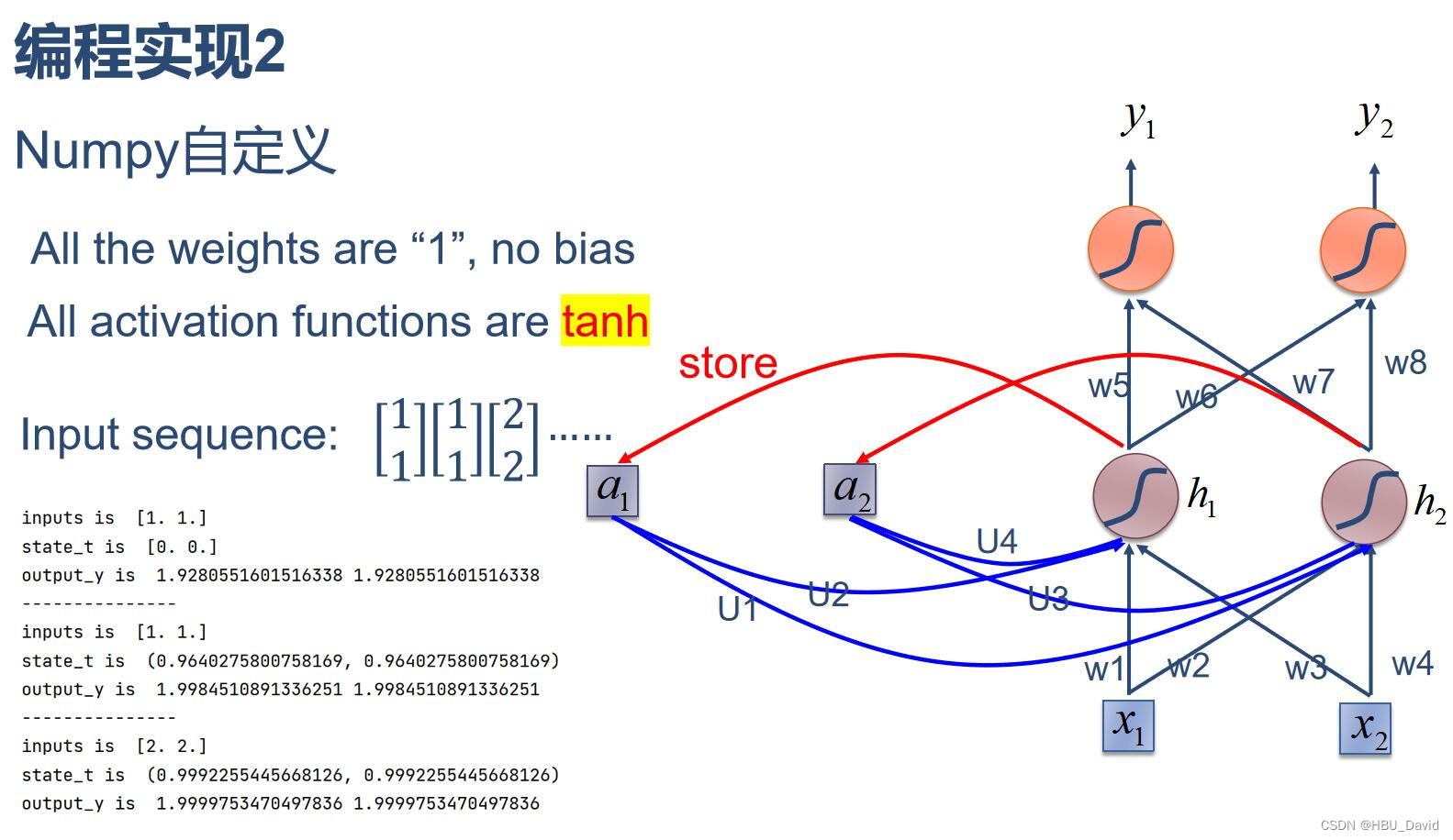
二、在1的基础上，增加激活函数tanh

import numpy as np
 
inputs = np.array([[1., 1.],
                   [1., 1.],
                   [2., 2.]])  # 初始化输入序列
print('inputs is ', inputs)
 
state_t = np.zeros(2, )  # 初始化存储器
print('state_t is ', state_t)
 
w1, w2, w3, w4, w5, w6, w7, w8 = 1., 1., 1., 1., 1., 1., 1., 1.
U1, U2, U3, U4 = 1., 1., 1., 1.
print('--------------------------------------')
for input_t in inputs:
    print('inputs is ', input_t)
    print('state_t is ', state_t)
    in_h1 = np.tanh(np.dot([w1, w3], input_t) + np.dot([U2, U4], state_t))
    in_h2 = np.tanh(np.dot([w2, w4], input_t) + np.dot([U1, U3], state_t))
    state_t = in_h1, in_h2
    output_y1 = np.dot([w5, w7], [in_h1, in_h2])
    output_y2 = np.dot([w6, w8], [in_h1, in_h2])
    print('output_y is ', output_y1, output_y2)
    print('---------------')

输出结果：

E:\Python\python.exe "E:/pythonProject/ceshi 2.py"
inputs is  [[1. 1.]
 [1. 1.]
 [2. 2.]]
state_t is  [0. 0.]
--------------------------------------
inputs is  [1. 1.]
state_t is  [0. 0.]
output_y is  1.9280551601516338 1.9280551601516338
---------------
inputs is  [1. 1.]
state_t is  (0.9640275800758169, 0.9640275800758169)
output_y is  1.9984510891336251 1.9984510891336251
---------------
inputs is  [2. 2.]
state_t is  (0.9992255445668126, 0.9992255445668126)
output_y is  1.9999753470497836 1.9999753470497836
---------------

Process finished with exit code 0

三、分别使用nn.RNNCell、nn.RNN实现SRN

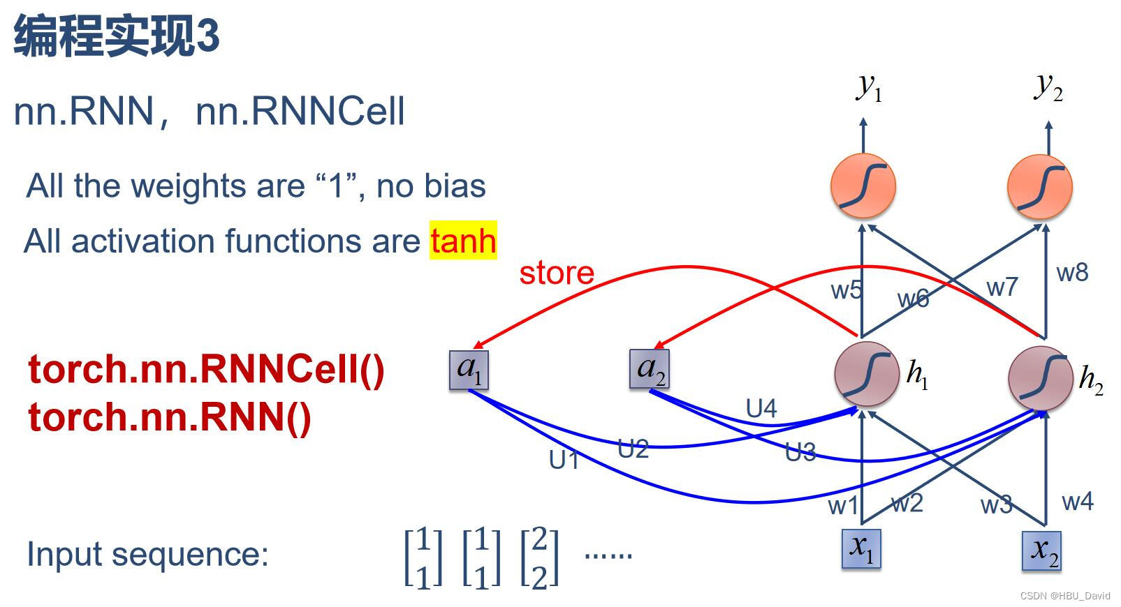
1、用torch.nn.RNNCell()

import torch
 
batch_size = 1
seq_len = 3  # 序列长度
input_size = 2  # 输入序列维度
hidden_size = 2  # 隐藏层维度
output_size = 2  # 输出层维度
 
# RNNCell
cell = torch.nn.RNNCell(input_size=input_size, hidden_size=hidden_size)
# 初始化参数 https://zhuanlan.zhihu.com/p/342012463
for name, param in cell.named_parameters():
    if name.startswith("weight"):
        torch.nn.init.ones_(param)
    else:
        torch.nn.init.zeros_(param)
# 线性层
liner = torch.nn.Linear(hidden_size, output_size)
liner.weight.data = torch.Tensor([[1, 1], [1, 1]])
liner.bias.data = torch.Tensor([0.0])
 
seq = torch.Tensor([[[1, 1]],
                    [[1, 1]],
                    [[2, 2]]])
hidden = torch.zeros(batch_size, hidden_size)
output = torch.zeros(batch_size, output_size)
 
for idx, input in enumerate(seq):
    print('=' * 20, idx, '=' * 20)
 
    print('Input :', input)
    print('hidden :', hidden)
 
    hidden = cell(input, hidden)
    output = liner(hidden)
    print('output :', output)

输出结果：

E:\Python\python.exe "E:/pythonProject/ceshi 2.py"
==================== 0 ====================
Input : tensor([[1., 1.]])
hidden : tensor([[0., 0.]])
output : tensor([[1.9281, 1.9281]], grad_fn=<AddmmBackward0>)
==================== 1 ====================
Input : tensor([[1., 1.]])
hidden : tensor([[0.9640, 0.9640]], grad_fn=<TanhBackward0>)
output : tensor([[1.9985, 1.9985]], grad_fn=<AddmmBackward0>)
==================== 2 ====================
Input : tensor([[2., 2.]])
hidden : tensor([[0.9992, 0.9992]], grad_fn=<TanhBackward0>)
output : tensor([[2.0000, 2.0000]], grad_fn=<AddmmBackward0>)

Process finished with exit code 0

nn.RNN实现:

E:\Python\python.exe "E:/pythonProject/ceshi 2.py"
out tensor([[[ 2.,  2.]],

        [[ 6.,  6.]],

        [[16., 16.]]], grad_fn=<StackBackward0>) tensor([[[16., 16.]]], grad_fn=<StackBackward0>)
Input : tensor([[1., 1.]])
hidden: 0 0
Output: tensor([[4., 4.]], grad_fn=<AddmmBackward0>)
--------------------------------------
Input : tensor([[1., 1.]])
hidden: tensor([[2., 2.]], grad_fn=<SelectBackward0>)
Output: tensor([[12., 12.]], grad_fn=<AddmmBackward0>)
--------------------------------------
Input : tensor([[2., 2.]])
hidden: tensor([[6., 6.]], grad_fn=<SelectBackward0>)
Output: tensor([[32., 32.]], grad_fn=<AddmmBackward0>)

Process finished with exit code 0

5. 实现“Character-Level Language Models”源代码（必做）

翻译Character-Level Language Models 相关内容

As a working example, suppose we only had a vocabulary of four possible letters “helo”, and wanted to train an RNN on the training sequence “hello”. This training sequence is in fact a source of 4 separate training examples: 1. The probability of “e” should be likely given the context of “h”, 2. “l” should be likely in the context of “he”, 3. “l” should also be likely given the context of “hel”, and finally 4. “o” should be likely given the context of “hell”.

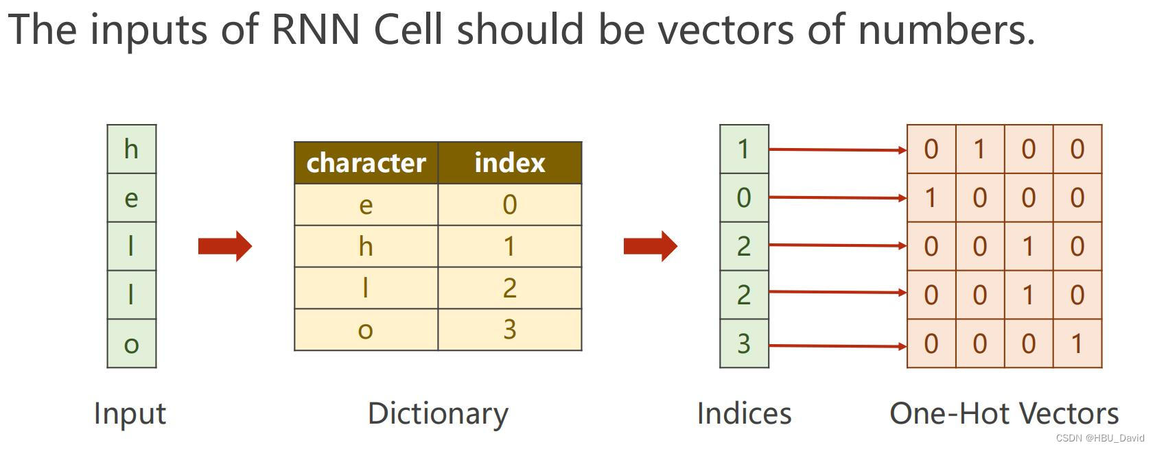
Concretely, we will encode each character into a vector using 1-of-k encoding (i.e. all zero except for a single one at the index of the character in the vocabulary), and feed them into the RNN one at a time with the step function. We will then observe a sequence of 4-dimensional output vectors (one dimension per character), which we interpret as the confidence the RNN currently assigns to each character coming next in the sequence. Here’s a diagram:

作为一个工作示例，假设我们只有四个可能的字母“helo”的词汇表，并且想要训练一个RNN训练序列“hello”。这个训练序列实际上是4个单独训练示例的来源：1.“e”的概率应该在“h”的上下文中很可能出现，2.“l”应该在“he”的上下文下很可能出现；3.“l”也应该在“hel”的语境下很可能会出现，最后4.“o”可能在“地狱”的上下文里出现。



具体地说，我们将使用k取1编码将每个字符编码为一个向量（即，除了词汇表中字符索引处的单个字符外，所有字符都为零），并使用步进函数将它们一次一个地输入RNN。然后，我们将观察一个4维输出向量序列（每个字符一个维度），我们将其解释为RNN当前为序列中下一个字符分配的置信度。下面是一个图表：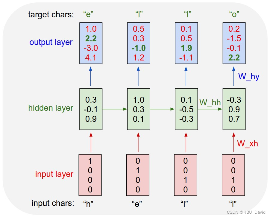

For example, we see that in the first time step when the RNN saw the character “h” it assigned confidence of 1.0 to the next letter being “h”, 2.2 to letter “e”, -3.0 to “l”, and 4.1 to “o”. Since in our training data (the string “hello”) the next correct character is “e”, we would like to increase its confidence (green) and decrease the confidence of all other letters (red). Similarly, we have a desired target character at every one of the 4 time steps that we’d like the network to assign a greater confidence to. Since the RNN consists entirely of differentiable operations we can run the backpropagation algorithm (this is just a recursive application of the chain rule from calculus) to figure out in what direction we should adjust every one of its weights to increase the scores of the correct targets (green bold numbers). We can then perform a parameter update, which nudges every weight a tiny amount in this gradient direction. If we were to feed the same inputs to the RNN after the parameter update we would find that the scores of the correct characters (e.g. “e” in the first time step) would be slightly higher (e.g. 2.3 instead of 2.2), and the scores of incorrect characters would be slightly lower. We then repeat this process over and over many times until the network converges and its predictions are eventually consistent with the training data in that correct characters are always predicted next.

例如，我们看到，在RNN看到字符“h”的第一个时间步骤中，它将置信度1.0分配给下一个字母“h”，2.2分配给字母“e”，-3.0分配给“l”，4.1分配给“o”。因为在我们的训练数据（字符串“hello”）中，下一个正确的字符是“e”，所以我们希望增加其置信度（绿色），并降低所有其他字母（红色）的置信度。类似地，我们希望网络为4个时间步骤中的每一个分配更大的置信度，我们都有一个期望的目标角色。由于RNN完全由可微操作组成，我们可以运行反向传播算法（这只是微积分中链式规则的递归应用），以确定我们应该向哪个方向调整每个权重，以增加正确目标的分数（绿色粗体数字）。然后，我们可以执行一个参数更新，在这个梯度方向上微调每个权重。如果我们在参数更新后将相同的输入馈送到RNN，我们会发现正确字符的分数（例如，第一时间步中的“e”）将略高（例如，2.3而不是2.2），而错误字符的分数将略低。然后，我们反复重复这个过程，直到网络收敛，其预测最终与训练数据一致，因为接下来总是预测正确的字符。

import numpy as np
import random
#utils.py中定义了本次实验所需要的辅助函数
#包括朴素RNN的前向/反向传播  和我们在上一个实验中实现的差不多
from utils import *
data = open('D:/dinos.txt', 'r').read() #读取dinos.txt中的所有恐龙名字 read()逐字符读取 返回一个字符串
data= data.lower()#把所有名字转为小写
chars = list(set(data))#得到字符列表并去重
print(chars)  #'a'-'z' '\n'  27个字符
data_size, vocab_size = len(data), len(chars)
print('There are %d total characters and %d unique characters in your data.' % (data_size, vocab_size))
char_to_ix = { ch:i for i,ch in enumerate(sorted(chars)) }
ix_to_char = { i:ch for i,ch in enumerate(sorted(chars)) }
print(ix_to_char)
 
def softmax(x):
    ''''softmax激活函数'''
    e_x = np.exp(x - np.max(x))  # 首先对输入做一个平移 减去最大值 使其最大值为0 再取exp 避免指数爆炸
    return e_x / e_x.sum(axis=0)
 
 
def smooth(loss, cur_loss):
    return loss * 0.999 + cur_loss * 0.001
 
 
def print_sample(sample_ix, ix_to_char):
    '''
    得到采样的索引对应的字符
    sample_ix:采样字符的索引
    ix_to_char:索引到字符的映射字典
    '''
    txt = ''.join(ix_to_char[ix] for ix in sample_ix)  # 连接成字符串
    txt = txt[0].upper() + txt[1:]  # 首字母大写
    print('%s' % (txt,), end='')
 
 
def get_initial_loss(vocab_size, seq_length):
    return -np.log(1.0 / vocab_size) * seq_length
 
 
def initialize_parameters(n_a, n_x, n_y):
    """
    用小随机数初始化模型参数
    Returns:
    parameters -- Python字典包含:
                        Wax -- 与输入相乘的权重矩阵, 维度 (n_a, n_x)
                        Waa -- 与之前隐藏状态相乘的权重矩阵, 维度 (n_a, n_a)
                        Wya -- 与当前隐藏状态相乘用于产生输出的权重矩阵, 维度(n_y,n_a)
                        ba --  计算当前隐藏状态的偏置参数  维度 (n_a, 1)
                        by --  计算当前输出的偏置参数  维度 (n_y, 1)
    """
    np.random.seed(1)
    Wax = np.random.randn(n_a, n_x) * 0.01
    Waa = np.random.randn(n_a, n_a) * 0.01
    Wya = np.random.randn(n_y, n_a) * 0.01
    b = np.zeros((n_a, 1))
    by = np.zeros((n_y, 1))
 
    parameters = {"Wax": Wax, "Waa": Waa, "Wya": Wya, "b": b, "by": by}
 
    return parameters
### GRADED FUNCTION: clip
 
def clip(gradients, maxValue):
    '''
    把每个梯度值剪切到 minimum 和 maximum之间.
    Arguments:
    gradients -- Python梯度字典 包含 "dWaa", "dWax", "dWya", "db", "dby"
    maxValue -- 每个大于maxValue或小于-maxValue的梯度值 被设置为该值
    Returns:
    gradients -- Python梯度字典 包含剪切后的切度
    '''
 
    # 取出梯度字典中存储的梯度
    dWaa, dWax, dWya, db, dby = gradients['dWaa'], gradients['dWax'], gradients['dWya'], gradients['db'], gradients[
        'dby']
 
    # 对每个梯度[dWax, dWaa, dWya, db, dby]进行剪切
    for gradient in [dWax, dWaa, dWya, db, dby]:
        # gradient[gradient>maxValue] = maxValue
        # gradient[gradient<-maxValue] = -maxValue
        np.clip(gradient, -maxValue, maxValue, out=gradient)
 
    gradients = {"dWaa": dWaa, "dWax": dWax, "dWya": dWya, "db": db, "dby": dby}
 
    return gradients
 
 
# GRADED FUNCTION: sample
 
def sample(parameters, char_to_ix, seed):
    """
    根据朴素RNN输出的概率分布对字符序列进行采样
    Arguments:
    parameters --Python字典 包含模型参数 Waa, Wax, Wya, by, and b.
    char_to_ix -- Python字典 把每个字符映射为索引
    seed -- .
    Returns:
    indices -- 包含采样字符索引的列表.
    """
 
    # 得到模型参数 和相关维度信息
    Waa, Wax, Wya, by, b = parameters['Waa'], parameters['Wax'], parameters['Wya'], parameters['by'], parameters['b']
    vocab_size = by.shape[0]  # 字典大小  输出单元的数量
    n_a = Waa.shape[1]  # 隐藏单元数量
 
    # Step 1: 创建第一个时间步骤上输入的初始向量 初始化序列生成
    x = np.zeros((vocab_size, 1))
    # Step 1': 初始化a_prev
    a_prev = np.zeros((n_a, 1))
 
    # 保存生成字符index的列表
    indices = []
 
    # 检测换行符, 初始化为 -1
    idx = -1
 
    # 在每个时间步骤上进行循环.在每个时间步骤输出的概率分布上采样一个字符
    # 把采样字典的index添加到indices中. 如果达到50个字符就停止 (说明模型训练有点问题)
    #  用于终止无限循环   模型如果训练的不错的话  在遇到换行符之前不会达到50个字符
    counter = 0
    newline_character = char_to_ix['\n']  # 换行符索引
 
    while (idx != newline_character and counter != 50):  # 如果生成的字符不是换行符且循环次数小于50  就继续
 
        # Step 2: 对x进行前向传播   公式(1), (2) and (3)
        a = np.tanh(Wax.dot(x) + Waa.dot(a_prev) + b)  # (n_a,1)
        z = Wya.dot(a) + by  # (n_y,1)
        y = softmax(z)  # (n_y,1)
 
        np.random.seed(counter + seed)
 
        # Step 3:从输出的概率分布y中 采样一个字典中的字符索引
        idx = np.random.choice(range(vocab_size), p=y.ravel())
        indices.append(idx)
 
        # Step 4: 根据采样的索引 得到对应字符的one-hot形式 重写输入x
        x = np.zeros((vocab_size, 1))
        x[idx] = 1
 
        # 更新a_prev
        a_prev = a
 
        seed += 1
        counter += 1
 
    if (counter == 50):
        indices.append(char_to_ix['\n'])
 
    return indices
 
 
def rnn_step_forward(parameters, a_prev, x):
    '''朴素RNN单元的前行传播'''
    # 从参数字典中取出参数
    Waa, Wax, Wya, by, b = parameters['Waa'], parameters['Wax'], parameters['Wya'], parameters['by'], parameters['b']
    # 计算当前时间步骤上的隐藏状态
    a_next = np.tanh(np.dot(Wax, x) + np.dot(Waa, a_prev) + b)
    # 计算当前时间步骤上的预测输出  通过一个输出层(使用softmax激活函数，多分类 ，类别数为字典大小)
    p_t = softmax(np.dot(Wya, a_next) + by)
 
    return a_next, p_t
 
 
def rnn_step_backward(dy, gradients, parameters, x, a, a_prev):
    '''朴素RNN单元的反向传播'''
    gradients['dWya'] += np.dot(dy, a.T)
    gradients['dby'] += dy
    da = np.dot(parameters['Wya'].T, dy) + gradients['da_next']  # backprop into h
    daraw = (1 - a * a) * da  # backprop through tanh nonlinearity
    gradients['db'] += daraw
    gradients['dWax'] += np.dot(daraw, x.T)
    gradients['dWaa'] += np.dot(daraw, a_prev.T)
    gradients['da_next'] = np.dot(parameters['Waa'].T, daraw)
    return gradients
 
 
def update_parameters(parameters, gradients, lr):
    '''
    使用随机梯度下降法更新模型参数
    parameters：模型参数字典
    gradients：对模型参数计算的梯度
    lr：学习率
    '''
    parameters['Wax'] += -lr * gradients['dWax']
    parameters['Waa'] += -lr * gradients['dWaa']
    parameters['Wya'] += -lr * gradients['dWya']
    parameters['b'] += -lr * gradients['db']
    parameters['by'] += -lr * gradients['dby']
    return parameters
 
 
def rnn_forward(X, Y, a0, parameters, vocab_size=27):
    '''朴素RNN的前行传播
    和上一个实验实验的RNN有所不同，之前我们一次处理m个样本/序列 要求m个序列有相同的长度
    本次实验的RNN，一次只处理一个样本/序列(名字单词) 所以不用统一长度。
     X -- 整数列表，每个数字代表一个字符的索引。 X是一个训练样本 代表一个单词
     Y -- 整数列表，每个数字代表一个字符的索引。 Y是一个训练样本对应的真实标签 为X中的索引左移一位
    '''
 
    # Initialize x, a and y_hat as empty dictionaries
    x, a, y_hat = {}, {}, {}
 
    a[-1] = np.copy(a0)
 
    # initialize your loss to 0
    loss = 0
 
    for t in range(len(X)):
 
        # 设置x[t]为one-hot向量形式.
        # 如果 X[t] == None, 设置 x[t]=0向量. 设置第一个时间步骤的输入为0向量
        x[t] = np.zeros((vocab_size, 1))  # 设置每个时间步骤的输入向量
        if (X[t] != None):
            x[t][X[t]] = 1  # one-hot形式 索引位置为1 其余为0
 
        # 运行一步RNN前向传播
        a[t], y_hat[t] = rnn_step_forward(parameters, a[t - 1], x[t])
        # 得到当前时间步骤的隐藏状态和预测输出
 
        # 把预测输出和真实标签结合 计算交叉熵损失
        loss -= np.log(y_hat[t][Y[t], 0])
 
    cache = (y_hat, a, x)
 
    return loss, cache
 
 
def rnn_backward(X, Y, parameters, cache):
    '''朴素RNN的反向传播'''
    # Initialize gradients as an empty dictionary
    gradients = {}
 
    # Retrieve from cache and parameters
    (y_hat, a, x) = cache
    Waa, Wax, Wya, by, b = parameters['Waa'], parameters['Wax'], parameters['Wya'], parameters['by'], parameters['b']
 
    # each one should be initialized to zeros of the same dimension as its corresponding parameter
    gradients['dWax'], gradients['dWaa'], gradients['dWya'] = np.zeros_like(Wax), np.zeros_like(Waa), np.zeros_like(Wya)
    gradients['db'], gradients['dby'] = np.zeros_like(b), np.zeros_like(by)
    gradients['da_next'] = np.zeros_like(a[0])
 
    ### START CODE HERE ###
    # Backpropagate through time
    for t in reversed(range(len(X))):
        dy = np.copy(y_hat[t])
        dy[Y[t]] -= 1
        gradients = rnn_step_backward(dy, gradients, parameters, x[t], a[t], a[t - 1])
    ### END CODE HERE ###
 
    return gradients, a
 
 
# GRADED FUNCTION: optimize
 
def optimize(X, Y, a_prev, parameters, learning_rate=0.01):
    """
    执行一步优化过程(随机梯度下降，一次优化使用一个训练训练).
    Arguments:
    X -- 整数列表，每个数字代表一个字符的索引。 X是一个训练样本 代表一个单词
    Y -- 整数列表，每个数字代表一个字符的索引。 Y是一个训练样本对应的真实标签 为X中的索引左移一位
    a_prev -- 上一个时间步骤产生的隐藏状态
    parameters -- Python字典包含:
                        Wax -- 与输入相乘的权重矩阵, 维度 (n_a, n_x)
                        Waa -- 与之前隐藏状态相乘的权重矩阵, 维度 (n_a, n_a)
                        Wya -- 与当前隐藏状态相乘用于产生输出的权重矩阵, 维度 (n_y, n_a)
                        ba --  计算当前隐藏状态的偏置参数  维度 (n_a, 1)
                        by --  计算当前输出的偏置参数  维度 (n_y, 1)
    learning_rate -- 学习率
    Returns:
    loss -- loss函数值(交叉熵)
    gradients -- python dictionary containing:
                        dWax -- Gradients of input-to-hidden weights, of shape (n_a, n_x)
                        dWaa -- Gradients of hidden-to-hidden weights, of shape (n_a, n_a)
                        dWya -- Gradients of hidden-to-output weights, of shape (n_y, n_a)
                        db -- Gradients of bias vector, of shape (n_a, 1)
                        dby -- Gradients of output bias vector, of shape (n_y, 1)
    a[len(X)-1] -- 最后一个隐藏状态 (n_a, 1)
    """
 
    # 通过时间前向传播
    loss, cache = rnn_forward(X, Y, a_prev, parameters, vocab_size=27)
 
    # 通过时间的反向传播
    gradients, a = rnn_backward(X, Y, parameters, cache)
 
    # 梯度剪切 -5 (min)  5 (max)
    gradients = clip(gradients, maxValue=5)
 
    # 更新参数
    parameters = update_parameters(parameters, gradients, lr=learning_rate)
 
    return loss, gradients, a[len(X) - 1]
 
 
# GRADED FUNCTION: model
 
def model(data, ix_to_char, char_to_ix, num_iterations=35000, n_a=50, dino_names=7, vocab_size=27):
    """
    训练模型生成恐龙名字.
    Arguments:
    data -- 文本语料(恐龙名字数据集)
    ix_to_char -- 从索引到字符的映射字典
    char_to_ix -- 从字符到索引的映射字典
    num_iterations -- 随机梯度下降的迭代次数  每次使用一个训练样本(一个名字)
    n_a -- RNN单元中的隐藏单元数
    dino_names -- 采样的恐龙名字数量
    vocab_size -- 字典的大小  文本语料中不同的字符数
    Returns:
    parameters --  训练好的参数
    """
 
    # 输入特征向量x的维度n_x, 输出预测概率向量的维度n_y  2者都为字典大小
    n_x, n_y = vocab_size, vocab_size
 
    # 初始化参数
    parameters = initialize_parameters(n_a, n_x, n_y)
 
    # 初始化loss (this is required because we want to smooth our loss, don't worry about it)
    loss = get_initial_loss(vocab_size, dino_names)
 
    # 得到所有恐龙名字的列表 (所有训练样本).
    with open("D:/dinos.txt") as f:
        examples = f.readlines()  # 读取所有行 每行是一个名字 作为列表的一个元素
    examples = [x.lower().strip() for x in examples]  # 转换小写 去掉换行符
 
    # 随机打乱所有恐龙名字 所有训练样本
    np.random.seed(0)
    np.random.shuffle(examples)
 
    # 初始化隐藏状态为0
    a_prev = np.zeros((n_a, 1))
 
    # 优化循环
    for j in range(num_iterations):
 
        # 得到一个训练样本 (X,Y)
        index = j % len(examples)  # 得到随机打乱后的一个名字的索引
        X = [None] + [char_to_ix[ch] for ch in examples[index]]  # 把名字中的每个字符转为对应的索引 第一个字符为None翻译为0向量
        Y = X[1:] + [char_to_ix['\n']]
 
        # 随机梯度下降 执行一次优化: Forward-prop -> Backward-prop -> Clip -> Update parameters
        # 学习率 0.01
        curr_loss, gradients, a_prev = optimize(X, Y, a_prev, parameters, learning_rate=0.01)
 
        # 使用延迟技巧保持loss平稳. 加速训练
        loss = smooth(loss, curr_loss)
 
        # 每2000次随机梯度下降迭代, 通过sample()生成'n'个字符(1个名字)  来检查模型是否训练正确
        if j % 2000 == 0:
 
            print('Iteration: %d, Loss: %f' % (j, loss) + '\n')
 
            seed = 0
            for name in range(dino_names):  # 生成名字的数量
 
                # 得到采样字符的索引
                sampled_indices = sample(parameters, char_to_ix, seed)
                # 得到索引对应的字符 生成一个名字
                print_sample(sampled_indices, ix_to_char)
 
                seed += 1  # To get the same result for grading purposed, increment the seed by one.
 
            print('\n')
 
    return parameters
parameters = model(data, ix_to_char, char_to_ix) #训练模型

这个模型训练花的时间太长，就略过了。

六、分析“序列到序列”源代码（选做）

# Model
class Seq2Seq(nn.Module):
    def __init__(self):
        super(Seq2Seq, self).__init__()
        self.encoder = nn.RNN(input_size=n_class, hidden_size=n_hidden, dropout=0.5) # encoder
        self.decoder = nn.RNN(input_size=n_class, hidden_size=n_hidden, dropout=0.5) # decoder
        self.fc = nn.Linear(n_hidden, n_class)
 
    def forward(self, enc_input, enc_hidden, dec_input):
        # enc_input(=input_batch): [batch_size, n_step+1, n_class]
        # dec_inpu(=output_batch): [batch_size, n_step+1, n_class]
        enc_input = enc_input.transpose(0, 1) # enc_input: [n_step+1, batch_size, n_class]
        dec_input = dec_input.transpose(0, 1) # dec_input: [n_step+1, batch_size, n_class]
 
        # h_t : [num_layers(=1) * num_directions(=1), batch_size, n_hidden]
        _, h_t = self.encoder(enc_input, enc_hidden)
        # outputs : [n_step+1, batch_size, num_directions(=1) * n_hidden(=128)]
        outputs, _ = self.decoder(dec_input, h_t)
 
        model = self.fc(outputs) # model : [n_step+1, batch_size, n_class]
        return model
 
model = Seq2Seq().to(device)
criterion = nn.CrossEntropyLoss().to(device)
optimizer = torch.optim.Adam(model.parameters(), lr=0.001)

解释：

7. “编码器-解码器”的简单实现

import torch
import numpy as np
import torch.nn as nn
import torch.utils.data as Data
 
device = torch.device('cuda' if torch.cuda.is_available() else 'cpu')
 
letter = [c for c in 'SE?abcdefghijklmnopqrstuvwxyz']
letter2idx = {n: i for i, n in enumerate(letter)}
 
seq_data = [['man', 'women'], ['black', 'white'], ['king', 'queen'], ['girl', 'boy'], ['up', 'down'], ['high', 'low']]
 
# Seq2Seq Parameter
n_step = max([max(len(i), len(j)) for i, j in seq_data])  # max_len(=5)
n_hidden = 128
n_class = len(letter2idx)  # classfication problem
batch_size = 3
 
 
def make_data(seq_data):
    enc_input_all, dec_input_all, dec_output_all = [], [], []
 
    for seq in seq_data:
        for i in range(2):
            seq[i] = seq[i] + '?' * (n_step - len(seq[i]))  # 'man??', 'women'
 
        enc_input = [letter2idx[n] for n in (seq[0] + 'E')]  # ['m', 'a', 'n', '?', '?', 'E']
        dec_input = [letter2idx[n] for n in ('S' + seq[1])]  # ['S', 'w', 'o', 'm', 'e', 'n']
        dec_output = [letter2idx[n] for n in (seq[1] + 'E')]  # ['w', 'o', 'm', 'e', 'n', 'E']
 
        enc_input_all.append(np.eye(n_class)[enc_input])
        dec_input_all.append(np.eye(n_class)[dec_input])
        dec_output_all.append(dec_output)  # not one-hot
 
    # make tensor
    return torch.Tensor(enc_input_all), torch.Tensor(dec_input_all), torch.LongTensor(dec_output_all)
 
enc_input_all, dec_input_all, dec_output_all = make_data(seq_data)
 
 
class TranslateDataSet(Data.Dataset):
    def __init__(self, enc_input_all, dec_input_all, dec_output_all):
        self.enc_input_all = enc_input_all
        self.dec_input_all = dec_input_all
        self.dec_output_all = dec_output_all
 
    def __len__(self):  # return dataset size
        return len(self.enc_input_all)
 
    def __getitem__(self, idx):
        return self.enc_input_all[idx], self.dec_input_all[idx], self.dec_output_all[idx]
 
 
loader = Data.DataLoader(TranslateDataSet(enc_input_all, dec_input_all, dec_output_all), batch_size, True)
 
 
# Model
class Seq2Seq(nn.Module):
    def __init__(self):
        super(Seq2Seq, self).__init__()
        self.encoder = nn.RNN(input_size=n_class, hidden_size=n_hidden, dropout=0.5)  # encoder
        self.decoder = nn.RNN(input_size=n_class, hidden_size=n_hidden, dropout=0.5)  # decoder
        self.fc = nn.Linear(n_hidden, n_class)
 
    def forward(self, enc_input, enc_hidden, dec_input):
        enc_input = enc_input.transpose(0, 1)  # enc_input: [n_step+1, batch_size, n_class]
        dec_input = dec_input.transpose(0, 1)  # dec_input: [n_step+1, batch_size, n_class]
 
        # h_t : [num_layers(=1) * num_directions(=1), batch_size, n_hidden]
        _, h_t = self.encoder(enc_input, enc_hidden)
        # outputs : [n_step+1, batch_size, num_directions(=1) * n_hidden(=128)]
        outputs, _ = self.decoder(dec_input, h_t)
 
        model = self.fc(outputs)  # model : [n_step+1, batch_size, n_class]
        return model
 
 
model = Seq2Seq().to(device)
criterion = nn.CrossEntropyLoss().to(device)
optimizer = torch.optim.Adam(model.parameters(), lr=0.001)
 
for epoch in range(5000):
    for enc_input_batch, dec_input_batch, dec_output_batch in loader:
        # make hidden shape [num_layers * num_directions, batch_size, n_hidden]
        h_0 = torch.zeros(1, batch_size, n_hidden).to(device)
 
        (enc_input_batch, dec_intput_batch, dec_output_batch) = (
        enc_input_batch.to(device), dec_input_batch.to(device), dec_output_batch.to(device))
        # enc_input_batch : [batch_size, n_step+1, n_class]
        # dec_intput_batch : [batch_size, n_step+1, n_class]
        # dec_output_batch : [batch_size, n_step+1], not one-hot
        pred = model(enc_input_batch, h_0, dec_intput_batch)
        # pred : [n_step+1, batch_size, n_class]
        pred = pred.transpose(0, 1)  # [batch_size, n_step+1(=6), n_class]
        loss = 0
        for i in range(len(dec_output_batch)):
            # pred[i] : [n_step+1, n_class]
            # dec_output_batch[i] : [n_step+1]
            loss += criterion(pred[i], dec_output_batch[i])
        if (epoch + 1) % 1000 == 0:
            print('Epoch:', '%04d' % (epoch + 1), 'cost =', '{:.6f}'.format(loss))
 
        optimizer.zero_grad()
        loss.backward()
        optimizer.step()
 
 
# Test
def translate(word):
    enc_input, dec_input, _ = make_data([[word, '?' * n_step]])
    enc_input, dec_input = enc_input.to(device), dec_input.to(device)
    # make hidden shape [num_layers * num_directions, batch_size, n_hidden]
    hidden = torch.zeros(1, 1, n_hidden).to(device)
    output = model(enc_input, hidden, dec_input)
    # output : [n_step+1, batch_size, n_class]
 
    predict = output.data.max(2, keepdim=True)[1]  # select n_class dimension
    decoded = [letter[i] for i in predict]
    translated = ''.join(decoded[:decoded.index('E')])
 
    return translated.replace('?', '')
 
print('test')
print('man ->', translate('man'))
print('mans ->', translate('mans'))
print('king ->', translate('king'))
print('black ->', translate('black'))
print('up ->', translate('up'))
print('old ->', translate('old'))
print('high ->', translate('high'))

输出结果：

Epoch: 1000 cost = 0.002507
Epoch: 1000 cost = 0.002449
Epoch: 2000 cost = 0.000532
Epoch: 2000 cost = 0.000495
Epoch: 3000 cost = 0.000154
Epoch: 3000 cost = 0.000160
Epoch: 4000 cost = 0.000056
Epoch: 4000 cost = 0.000051
Epoch: 5000 cost = 0.000019
Epoch: 5000 cost = 0.000019
test
man -> women
mans -> women
king -> queen
black -> white
up -> down
old -> white
high -> low

Process finished with exit code 0

总结：

主要是了解了char-RNN模型，对比了nn.RNN（）和nn.RNNCell（）的不同，但是我自己感觉还是一知半解，有待之后好好看看，研究一下。，