边缘检测门限化分割霍夫变换区域分割

最新推荐文章于 2021-08-03 17:30:37 发布

ChiruZy

最新推荐文章于 2021-08-03 17:30:37 发布

阅读量794

点赞数 1

分类专栏：数字图像处理文章标签：边缘检测 python 卷积

本文链接：https://blog.csdn.net/weixin_51917840/article/details/116720043

版权

数字图像处理专栏收录该内容

2 篇文章 0 订阅

订阅专栏

边缘检测门限化分割霍夫变换区域分割

0. 通用函数定义

在本次作业中，将会多次使用到卷积、梯度合成、阈值分割以及图片批量显示的操作，故将这些操作定义为函数，以便重复使用。

- 卷积

def conv_process(img, operators, k_size):
    space = k_size // 2
    raw = np.pad(img, [space, space], 'edge')
    w, h = raw.shape

    res = [np.zeros(img.shape) for _ in range(len(operators))]
    for row in range(space, w - space):
        for col in range(space, h - space):
            for g, o in zip(res, operators):
                block = raw[row - space:row + space + 1, 
                            col - space:col + space + 1]
                g[row - space, col - space] = np.sum(block * o)
    return res

该函数设置了三个参数，分别为需要卷积的图片，一组卷积操作的算子/模板，算子的尺寸。
首先根据算子的尺寸将图像边缘填充到合适的尺寸。再通过滑动窗口，将每个算子对图像进行卷积，最后将结果返回。

- 梯度合成

def get_edge_gradient(gs):
    gs = np.abs(np.array(gs))
    return gs.max(axis=0)

函数接收一组梯度，将所有方向的梯度在 z 轴堆叠后，对其进行绝对值操作，然后以该轴取最大值即可。

- 图片批量显示

def plot_imgs(row, col, imgs, titles):
    for idx, (img, title) in enumerate(zip(imgs, titles)):
        plt.subplot(row, col, idx + 1)
        plt.title(title)
        plt.imshow(img, cmap='gray')
        plt.axis('off')
    plt.show()

函数调用 matplotlib 用于批量输出图片，参数分别为图像一共有几行几列，以及图像序列与图像的标题序列。

- 单阈值分割

def threshold_seg(g, thres):
    g = (g - np.min(g)) / (np.max(g) - np.min(g)) * 255
    return np.where(g > thres, 255, 0).astype('uint8')

函数接收一张图片与一个阈值，首先将该图片标准化到 0~255 的区间，再使用传入的阈值对图像的每个点的值映射到 0 或 255。

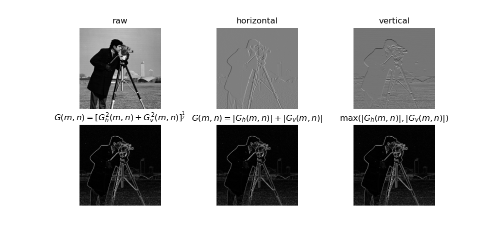
1. 用正交梯度法实现边缘点检测

已知水平方向和垂直方向的梯度可以定义为差分操作：
$\begin{cases} G_h(m,n) = f(m,n) - f(m, n-1) \\[0.5em] G_v(m,n) = f(m,n) - f(m-1, n) \end{cases}$
则水平和垂直方向的梯度模板代码如下：

def gradient_operator():
    W_h = np.array([[0, 0, 0], [-1, 1, 0], [0, 0, 0]])
    W_v = np.array([[0, -1, 0], [0, 1, 0], [0, 0, 0]])
    return W_h, W_v

使用 $W_h$ 和 $W_v$ 对图像进行卷积操作即可得到水平和垂直方向的梯度 $G_h$ 和 $G_v$ ，代码如下：

img = np.array(Image.open('cameraman.tif').convert('L')) / 255
G_h, G_v = conv_process(img, gradient_operator(), 3)
G1 = np.sqrt(G_v ** 2 + G_h ** 2)
G2 = np.abs(G_v) + np.abs(G_h)
G3 = np.maximum(np.abs(G_v), np.abs(G_h))

再使用三种不同的方法将梯度合成，如上方代码中的 $G_1$ , $G_2$ , $G_3$ 。正交梯度法边缘检测的结果如下图：

2. 五种梯度算子的边缘点检测实例

正交梯度算子已在上题中定义，Roberts 算子的定义代码如下：

def Roberts():
    W_h = np.array([[-1, 0, 0], [0, 1, 0], [0, 0, 0]])
    W_v = np.array([[0, -1, 0], [1, 0, 0], [0, 0, 0]])
    return W_h, W_v

Prewitt，Sobel， 各向同性Sobel 的垂直算子均可以通过水平算子顺时针旋转 90° 得到，代码如下：

def Prewitt():
    W_h = np.array([[-1, 0, 1], [-1, 0, 1], [-1, 0, 1]]) / 3
    return W_h, np.rot90(W_h)

def Sobel():
    W_h = np.array([[-1, 0, 1], [-2, 0, 2], [-1, 0, 1]]) / 4
    return W_h, np.rot90(W_h)
    
def Isotropic_Sobel():
    W_h = np.array([[-1, 0, 1], [-2**0.5, 0, 2**0.5], [-1, 0, 1]]) / (2 + 2**0.5)
    return W_h, np.rot90(W_h)

分别使用以上的算子对图像进行卷积操作，并使用 $\operatorname{MAX}_{i=0}^{N-1}(|G_i(m,n)|)$ 的梯度合成方法进行边缘检测：

img = np.array(Image.open('cameraman.tif').convert('L')) / 255
gradient = get_edge_gradient(conv_process(img, gradient_operator(), 3))
roberts = get_edge_gradient(conv_process(img, Roberts(), 3))
prewitt = get_edge_gradient(conv_process(img, Prewitt(), 3))
sobel = get_edge_gradient(conv_process(img, Sobel(), 3))
isotropic_Sobel = get_edge_gradient(conv_process(img, Isotropic_Sobel(), 3))

plot_imgs(2, 3, [img, gradient, roberts, prewitt, sobel, isotropic_Sobel],
              	['raw', 'gradient', 'Roberts', "Prewitt", "Sobel", 'Isotropic Sobel'])
plt.show()

结果如下图：
在这里插入图片描述

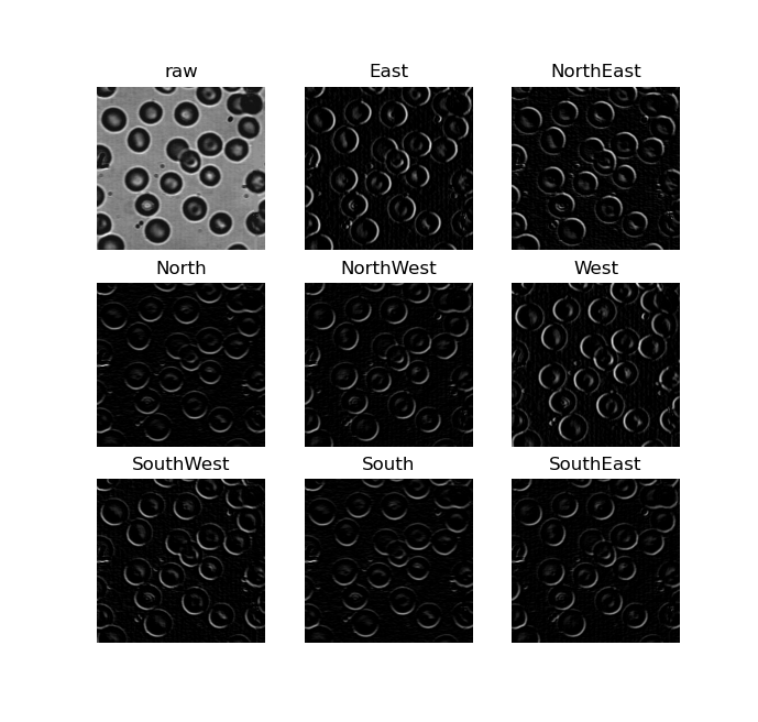
3. 8 方向梯度模板处理结果

8 方向梯度模板是由 Prewitt 模板旋转得到的，同时可以发现，南方向为东方向旋转 90° 得到，西方向又可以通过南方向旋转 90° 得到，东北方向可以通过西北方向旋转 90° 得到，东南方向又是西北方向乘以 -1。按此规律可以方便地得到所有 8 个方向的梯度模板：

def Prewitt_dirction():
    W_e = np.array([[-1, 0, 1], [-1, 0, 1], [-1, 0, 1]]) / 3
    W_en = np.array([[0, 1, 1], [-1, 0, 1], [-1, -1, 0]]) / 3
    W_s = np.rot90(W_e)
    W_es = np.rot90(W_en)
    return W_e, W_en, -W_s, -W_es, -W_e, -W_en, -W_s, -W_es

使用这组梯度模板对图像进行卷积操作，并将负梯度置零，即可得到图像在这八个方向上的梯度。代码如下：

img = np.array(Image.open('thresholded_image.jpg').convert('L')) / 255
gs = np.array(conv_process(img, Prewitt_dirction(), 3))
gs[gs < 0] = 0
plot_imgs(3, 3, [img, *gs], ['raw', 'East', 'NorthEast', 'North', 'NorthWest',
                             'West', 'SouthWest', 'South', 'SouthEast'])
plt.show()

八个方向的梯度图像如下：

4. 几种梯度算子的边缘点检测结果

Prewitt 算子、 Sobel 算子以及平均差分方向梯度算子已经在第二题和第三题中定义。而 Sobel 加权平均差分算子和 Kirsch 方向算子则与平均差分方向梯度算子的定义方法类似，都是将一个算子进行旋转得到的。其代码定义方法也与平均差分方向算子类似。只需要定义其中两个方向即可通过旋转和正负操作，直接得到其他方向：

def Sobel_dirction():
    W_e = np.array([[-1, 0, 1], [-2, 0, 2], [-1, 0, 1]]) / 4
    W_en = np.array([[0, 1, 2], [-1, 0, 1], [-2, -1, 0]]) / 4
    W_s = np.rot90(W_e)
    W_es = np.rot90(W_en)
    return W_e, W_en, -W_s, -W_es, -W_e, -W_en, -W_s, -W_es

def Kirsch_dirction():
    W_e  = np.array([[-3, -3,  5], [-3, 0,  5], [-3, -3,  5]]) / 15
    W_en = np.array([[-3,  5,  5], [-3, 0,  5], [-3, -3, -3]]) / 15
    W_s = np.rot90(W_e)
    W_w = np.rot90(W_s)
    W_n = np.rot90(W_w)
    W_es = np.rot90(W_en)
    W_ws = np.rot90(W_es)
    W_wn = np.rot90(W_ws)
    return W_e, W_en, W_n, W_wn, W_w, W_ws, W_s, W_es

使用以上的算子对图像进行卷积操作，并进行梯度合成，代码如下：

img = np.array(Image.open('cameraman.tif').convert('L')) / 255
prewitt = get_edge_gradient(conv_process(img, Prewitt(), 3))
sobel = get_edge_gradient(conv_process(img, Sobel(), 3))
ave_diff = get_edge_gradient(conv_process(img, Prewitt_dirction(), 3))
weighted_diff = get_edge_gradient(conv_process(img, Sobel_dirction(), 3))
Kirsch = get_edge_gradient(conv_process(img, Kirsch_dirction(), 3))

plot_imgs(2, 3, [img, prewitt, sobel, ave_diff, weighted_diff, Kirsch],
          ['raw', 'Prewitt', 'Sobel', 'Average difference\ndirection gradient',
           'Weighted difference\ndirection gradient', 'Kirsch'])
plt.show()

结果如下图所示：
在这里插入图片描述

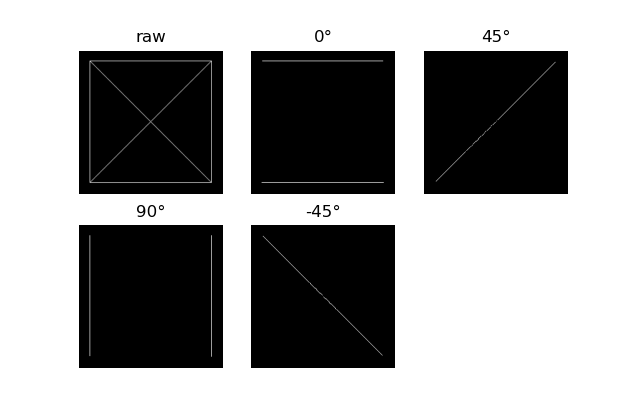
5. 基于线检测模板的检测示例

首先定义检测四个方向直线的方向模板，90° 模板可以由 0° 的模板旋转得到，135°模板也可以由 45° 模板旋转得到，如代码：

def line_detection_operator():
    W0 = np.array([[-1, -1, -1], [ 2, 2,  2], [-1, -1, -1]]) / 6
    W1 = np.array([[-1, -1,  2], [-1, 2, -1], [ 2, -1, -1]]) / 6
    return W0, W1, W0.T, np.rot90(W1)

使用这两个模板对图像进行卷积操作。由于噪声的影响，还对其做了阈值分割操作，对结果进行过滤，代码如下：

img = np.array(Image.open('line.png').convert('L')) / 255
res = threshold_seg(conv_process(img, line_detection_operator(), 3), 155)

plot_imgs(2, 3, [img, *res], ['raw', '0°', '45°', '90°', '-45°'])
plt.show()

结果如下图所示：

6. Laplacian 算子和 LoG 算子处理后的结果对比

根据 Laplacian 算子的定义可以得到以下代码：

def laplacian_operator(mode=4):
    assert mode in (4, 8)
    if mode == 4:
        return np.array([[0, -1, 0], [-1, 4, -1], [0, -1, 0]]),
    else:
        return np.array([[-1, -1, -1], [-1, 8, -1], [-1, -1, -1]]),

通过参数可以选择获取四邻域或八邻域的 Laplacian 算子。

LoG 算子为先对图像进行平滑操作，再使用 Laplacian 算子进行卷积操作。通过公式推导可以将两步结合，算子公式为：
$\frac{r^2 - 2\sigma^2}{\sigma^4}\exp({-\frac{r^2}{2\sigma^2}})$
根据公式可以写出代码：

def LoG(sigma, size=3):
    r, c = np.mgrid[0:size:1, 0:size:1]
    r -= int((size-1)/2)
    c -= int((size-1)/2)
    sigma2 = sigma ** 2
    sigma4 = sigma ** 4
    norm2 = r ** 2 + c ** 2
    kernel = (norm2 / sigma4 - 2/sigma2) * np.exp(- norm2 / (2 * sigma2))
    return kernel - np.mean(kernel),

代码的最后算子减去其均值，让其均值为 0。

分别使用四邻域 Laplacian 算子、八邻域 Laplacian 算子以及 LoG 算子对图像进行卷积操作，并使用合适的阈值进行分割，代码如下：

img = np.array(Image.open('cameraman.tif').convert('L')) / 255
laplacian4 = threshold_seg(conv_process(img, laplacian_operator(4), 3)[0], 160)
laplacian8 = threshold_seg(conv_process(img, laplacian_operator(8), 3)[0], 140)
log = threshold_seg(conv_process(img, LoG(0.6, 11), 11)[0], 145)

plot_imgs(2, 2, [img, laplacian4, laplacian8, log], ['raw', 'Laplacian_4', 'Laplacian_8', 'LoG'])
plt.show()

在这里插入图片描述

7. Hough 变换检测直线和圆的示例

(0) 提取边缘

在进行霍夫变换之前，需要先对图像进行边缘提取，并将结果进行阈值分割和二值化操作。以上的操作是由于霍夫变换是一个较为耗时的算法，需要遍历图像中的点并进行计算。经过边缘提取和阈值分割之后，可以过滤掉很大一部分不在直线上的点，从而减少计算量。此处使用了 Sobel 算子，进行边缘提取，代码如下:

img = np.array(Image.open('hough.png').convert('L'))
sobel_img = get_edge_gradient(conv_process(img, Sobel(), 3))
binary = threshold_seg(sobel_img, 140)

(1) Hough 线变换

已知一条直线在极坐标中可以表示为：
$\rho = x\cos\theta + y\sin\theta$
则一组 $(\rho, \theta)$ 可以唯一确定一条直线，所有可能的 $(\rho, \theta)$ 则组成了一个参数空间。Hough 线变换就是遍历原图中的每一个边缘点，对过该点的所有直线，在参数空间进行计数投票，最后计数最高的即为最有可能的那条线，实现代码如下：

def hough_line_transform(binary_img):
    w, h = binary_img.shape
    max_len = int(round(np.sqrt(w ** 2 + h ** 2)))
    thetas = np.deg2rad(np.linspace(-180, 0, 2*max_len))
    rhos = np.linspace(-max_len, max_len, 2*max_len)

    cos_t = np.cos(thetas)
    sin_t = np.sin(thetas)
    n_thetas = len(thetas)
    accumulator = np.zeros((2*max_len, n_thetas), dtype=np.int16)
    y_idxs, x_idxs = np.nonzero(binary_img > 0)

    for i in range(len(x_idxs)):
        x = x_idxs[i]
        y = y_idxs[i]

        for t_idx in range(n_thetas):
            rho = max_len + int(round(x * cos_t[t_idx] + y * sin_t[t_idx]))
            accumulator[rho, t_idx] += 1
    return accumulator, thetas, rhos

该函数的参数为步骤0中生成的二值化图像，函数中首先生成了所有可能的 $\rho$ 和 $\theta$ ，并缓存了 $\cos \theta$ 和 $\sin \theta$ 避免重复计算，然后生成了对应数量的累加器。接着遍历二值图像中的所有可能点，使用极坐标直线公式计算出所有过该点的直线的参数 $\rho$ 和 $\theta$ 。最后返回累加器和 $\rho$ 和 $\theta$ 数组。

(2) 直线还原与绘制

def unpack_hough_line(hough_line, t, r, shape):
    hough_line = (hough_line - np.min(hough_line)) / (np.max(hough_line) - np.min(hough_line)) * 255
    ls = np.argsort(hough_line.flatten())[-3:]

    lines = np.zeros(shape, dtype=np.uint8)
    kbs = []
    for l in ls:
        ir, it = np.unravel_index(l, hough_line.shape)
        rho, theta = r[ir], t[it]
        k = -np.cos(theta) / np.sin(theta)
        b = rho / np.sin(theta)
        kbs.append((k, b))

    for i in range(len(kbs)):
        k0, b0 = kbs[i]
        cross = []
        for idx, (k, b) in enumerate(kbs):
            if idx == i:
                continue
            cross.append(int(round((b - b0) / (k0 - k))))
        line = np.array([int(round(k0 * x + b0)) for x in range(img.shape[0])])
        lines[line[min(cross):max(cross)], list(range(min(cross), max(cross)))] = 255
    return lines

首先，根据先验知识可以得知原图中具有三条直线，则累加器中的前三个最大值所在位置对应的 $\rho$ 和 $\theta$ ，即为这三条直线方差的参数。

第二步，根据获得的 $\rho$ 和 $\theta$ ，可以通过公式计算得出直线在笛卡尔坐标系下的方程 $y = k x + b$ 的参数 $k$ 和 $b$ ，如第5~12行所示。再通过公式 $k_1 - k_2)x +(b_1 -b_2) = y$ 可以计算出这三条直线相交的点，如第14~20行所示。

最后在空白的数组上绘制出三条直线即可，如第21~23行所示。

(3) Hough 圆变换

已知圆在极坐标下可表示为：
$r\cos \theta \\ b = y - r\sin \theta$
其中 $(a, b)$ 为圆心坐标， $(x, y)$ 为圆上任何一点坐标， $r$ 为圆的半径。则一组参数 $(a, b, r)$ 即可唯一确定一个圆。霍夫圆变换的原理与霍夫线边换类似，只不过将参数空间从二维变成了三维。已知原图像上的某一点 $(x, y)$ ，就可以通过公式遍历出所有可能经过该点的圆的圆心以及半径，即所有可能的参数 $(a, b, r)$ ，最后通过统计即可得到图像上所有点可能经过的次数最多的那个圆的参数。代码如下：

def hough_circle_transform(binary_img, r_min, r_max):
    w, h = binary_img.shape

    max_len = int(round(np.sqrt(w ** 2 + h ** 2)))
    thetas = np.deg2rad(np.linspace(0, 360, 100))
    rhos = np.linspace(0, max_len, 100)
    radius = np.arange(r_min, r_max)

    cos_t = np.cos(thetas)
    sin_t = np.sin(thetas)
    n_thetas = len(thetas)
    n_radius = len(radius)

    accumulator = np.zeros((w, h, n_radius), dtype=np.int16)
    y_idxs, x_idxs = np.nonzero(binary_img > 0)

    for i in range(len(x_idxs)):
        x = x_idxs[i]
        y = y_idxs[i]
        for t_idx in range(n_thetas):
            for rho in rhos:
                a = int(round(x - rho * cos_t[t_idx]))
                b = int(round(y - rho * sin_t[t_idx]))
                r = int(round(np.sqrt((a - x) ** 2 + (b - y) ** 2)))
                if a < 0 or a >= w or b <0 or b>=h or r >= r_max or r < r_min:
                    continue
                accumulator[a, b, r-r_min] += 1
    return accumulator

代码上与线变换基本相同，多套了一层循环，从遍历每个点所有可能的 $\theta$ 来计算对应的 $\rho$ ，变为了遍历每个点所有的可能的 $\theta$ 和 $\rho$ 来计算对应的 $(a, b, r)$ 。参数 r_min 和 r_max 用于过滤掉半径过小或过大的圆。最后返回累加器，累加器中最大的位置所对应的 $(a, b, r)$ ，即为检测到的圆的圆心坐标和半径。

(4) 圆绘制

def draw_circle(shape, center, r):
    img = np.zeros(shape)
    theta = np.linspace(0, 2 * np.pi, 360)
    a, b = center
    for t in theta:
        x = int(round(a + r * np.cos(t)))
        y = int(round(b + r * np.sin(t)))
        img[x, y] = 255
    return img

根据已有的圆心和半径信息，使用圆的极坐标公式，在原图尺寸的空白数组中绘制圆。

(5) 具体步骤

img = np.array(Image.open('hough.png').convert('L'))
sobel_img = get_edge_gradient(conv_process(img, Sobel(), 3))

binary = threshold_seg(sobel_img, 140)
hough_line, t, r = hough_line_transform(binary)
lines = unpack_hough_line(hough_line, t, r, img.shape)

binary = threshold_seg(sobel_img, 80)
r_min, r_max = 10, 200
hough_circle = hough_circle_transform(binary, r_min, r_max)
x, y, r = np.unravel_index(np.argmax(hough_circle), hough_circle.shape)
circle = draw_circle(img.shape, (x, y), r+r_min)

hough = np.zeros(img.shape)
hough[(circle > 0) | (lines > 0)] = 255

plot_imgs(2, 4, [img, sobel_img, hough_line, lines, hough_circle.sum(axis=-1), circle, hough],
          ['raw', 'sobel', 'hough line transform', 'line detection', 'hough circle transform', 
           'circle detection', 'hough detection'])
plt.show()

以上代码中 1~12 行即为(0)~(4)中描述的步骤，14 ~ 15 行将线检测和圆检测的结果进行融合，最后输出图像:

在这里插入图片描述

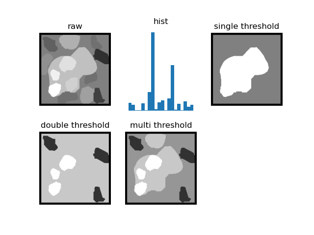
8. 门限化分割

（1）单阈值，双阈值，多阈值分割

此处将单阈值、双阈值、多阈值分割抽象为同一函数，如下：

def threshold_seg(img, thresholds):
    masks = [img <= thresholds[0]]
    for i in range(len(thresholds) - 1):
        masks.append((img > thresholds[i]) & (img <= thresholds[i+1]))
    masks.append(img > thresholds[-1])
    return masks

函数接收一张图片，以及一组阈值，通过遍历阈值的区间，输出 阈值数量 + 1 个 mask。

得到一组 mask 之后，可以通过这些 mask 对原图进行分割上色，代码如下：

def recolor(masks, colors=None, pad=6):
    if colors is None:
        colors = [i * (255 // (len(masks) + 1)) for i in range(1, len(masks)+1)]
    assert len(colors) == len(masks)
    img = np.zeros(masks[0].shape)
    for mask, c in zip(masks, colors):
        img[mask] = c
    img = np.pad(img, [pad, pad], 'constant', constant_values=(0, 0))
    return img

该函数接收一组 mask ，和一组颜色 colors，将原图中每个 mask 的区域映射为对应的颜色。color 为可选参数，若 color 为 None，则通过计算 mask 的数量，在 0~255 的范围中平均分配每个 mask 所在区域的颜色。

单阈值，双阈值以及多阈值分割的具体操作代码如下：

def simple_threshold_seg():
    img = np.array(Image.open('threshold_seg.jpg').convert('L'))
    plt_show_img((2, 3, 1), 'raw', img=np.pad(img, [6, 6], 'constant', constant_values=(0, 0)))
    plt_show_img((2, 3, 2), 'hist', hist=img.flatten(), bins=20)

    single = threshold_seg(img, [180])
    plt_show_img((2, 3, 3), 'single threshold', img=recolor(masks=single))
    double = threshold_seg(img, [105, 220])
    plt_show_img((2, 3, 4), 'double threshold', img=recolor(masks=double))
    multi = threshold_seg(img, [105, 170, 220])
    plt_show_img((2, 3, 5), 'multi threshold', img=recolor(masks=multi))
    plt.show()

结果如下：

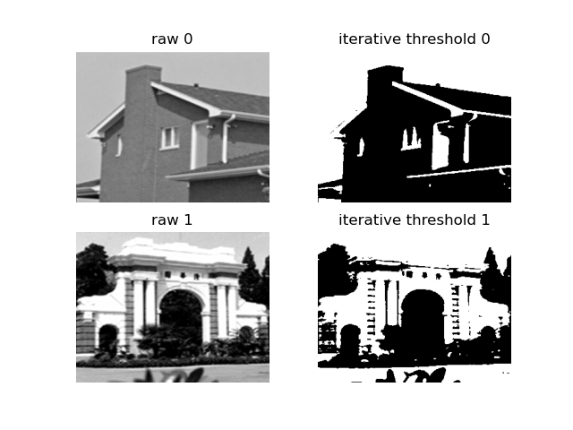
（2）迭代阈值法

迭代阈值法的方法是通过阈值将图像分为两个区域，并计算两个区域的灰度均值，对均值进行平均从而得到新的阈值，不断重复此项过程直至收敛。具体代码如下：

def iterative_threshold_method(max_iter=100, eps=1e-3):
    img0 = np.array(Image.open('building0.png').convert('L')) / 255.
    img1 = np.array(Image.open('building1.png').convert('L')) / 255.
    for idx, img in enumerate([img0, img1]):
        thres = (np.min(img) + np.max(img)) / 2
        for _ in range(max_iter):
            next = (np.mean(img[img > thres]) + np.mean(img[img <= thres])) / 2
            if abs(next - thres) < eps:
                break
            thres = next
        masks = threshold_seg(img, [thres])
        plt_show_img((2, 2, 1 + idx * 2), f'raw {idx}', img=img)
        plt_show_img((2, 2, 2 + idx * 2), f'iterative threshold {idx}',
                     img=recolor(masks=masks, color=[0, 255], pad=0))
    plt.show()

设置初始均值为整张图灰度最小值和最大值的平均值，如代码第 5 行所示。接着在迭代到最大迭代次数之前，不断地将图像按阈值进行分割，再计算两个区域平均灰度的平均值作为新的阈值，直到阈值的变化小于设定的最小值 eps，如代码 6~10 行所示。最后显示结果图像，如图：

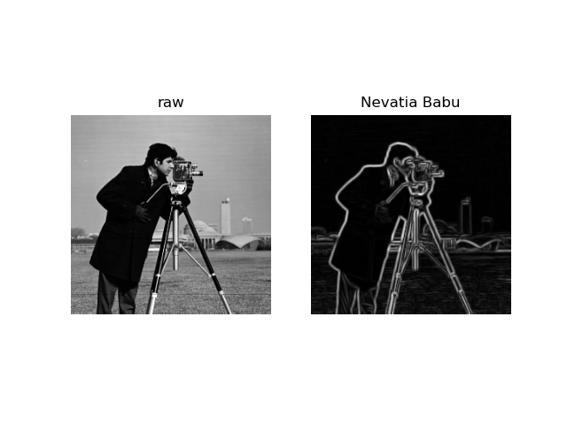
9. 12 方向梯度算子的边缘点检测结果

定义 12 方向梯度算子，12 方向梯度算子与之前的 8 方向梯度算子类似，都是通过旋转得到的。只要写出其中两个方向，再通过旋转和取负即可得到所有方向的算子，如代码：

def Nevatia_Babu():
    w0 = np.ones((5, 5))
    w0 *= np.array([-100, -100, 0, 100, 100]) / 1000
    w270 = np.rot90(w0)
    w180 = np.rot90(w270)
    w90 = np.rot90(w180)
    w60 = np.array([[100] * 5, [-32, 78, 100, 100, 100], 
                    [-100, -92, 0, 92, 100], 
    				[-100, -100, -100, -78, 32], 
                    [-100] * 5]) / 1102
    w330 = np.rot90(w60)
    w240 = np.rot90(w330)
    w150 = np.rot90(w240)
    w30 = -w60.T
    w300 = np.rot90(w30)
    w210 = np.rot90(w300)
    w120 = np.rot90(w210)
    return w0, w30, w60, w90, w120, w150, w180, w210, w240, w270, w300, w330

具体操作如下:

img = np.array(Image.open('cameraman.tif').convert('L')) / 255
nevatia_babu = get_edge_gradient(conv_process(img, Nevatia_Babu(), 5))
plot_imgs(1, 2, [img, nevatia_babu], ['raw', 'Nevatia Babu'])
plt.show()

结果如下：

10. 四叉树分裂合并法

四叉树分裂合并法分为两个步骤：

分裂：分裂操作即为判断图片是否符合某一准则，若符合则可以认为该图片只有一个区域。若不符合则需要将图片平均分成四个区域，然后分别对每一个小区域再进行判断。如此不断递归直至图片的区域不能再增多，即完成了分裂步骤。
合并：合并操作需要对每一个区域与其相邻的区域再进行准则判断，若符合该准则，则认为这两个区域能够被合并为同一区域，则将该两个区域标记为同一区域。反复进行该操作直至图像上所有像素不能再合并。

分裂的代码如下：

def quadtree_seg(img, seg, thres=10):
    if img.size == 0:
        return
    if np.var(img) < thres:
        if not hasattr(quadtree_seg, 'count'):
            quadtree_seg.count = 0
        seg[:, :] = quadtree_seg.count
        quadtree_seg.count += 1
        return
    w, h = img.shape
    quadtree_seg(img[0:w // 2, 0:h // 2], seg[0:w // 2, 0:h // 2], thres)
    quadtree_seg(img[w // 2:, 0:h // 2], seg[w // 2:, 0:h // 2], thres)
    quadtree_seg(img[0:w // 2, h // 2:], seg[0:w // 2, h // 2:], thres)
    quadtree_seg(img[w // 2:, h // 2:], seg[w // 2:, h // 2:], thres)

此处采用的准则为方差是否小于给定值，函数使用递归的写法，若该区域的方差不小于给定值，则将该区域分成四块，再对每块使用该函数判断、分割。若该区域方差小于给定值，则不进行分割，对该区域进行标记后直接返回。

合并的代码如下：

def merge(img, seg, thres=10, max_iter=100):
    merge = seg.copy()
    w, h = img.shape
    for _ in range(max_iter):
        merged = False
        for row in range(w - 1):
            for col in range(h - 1):
                v0 = merge[row, col]
                v1 = merge[row, col + 1]
                v2 = merge[row + 1, col]
                for v in v1, v2:
                    if v0 != v  and np.var(img[(merge == v0) | (merge == v )]) < thres:
                        merge[merge == v ] = v0
                        merged = True
        if not merged:
            break
    return merge

合并的代码第 4 行设置了最大迭代次数，防止死循环。第 5 行设置了一个参数 merged ，若本次循环中没有进行合并，则说明合并完成，将会退出循环。而第 6~14 行中，遍历了分割结果中所有的像素，并对右方和下方的区域进行比较，若右方或下方区域的标记与当前像素的标记不同，同时两个区域的方差又满足小于给定值的条件，将会把右方或下方区域的标记重新设定为与当前像素相同的值。

调用操作如下：

img = np.array(Image.open('thresholded_image.png').convert('L'))
seg = np.zeros(img.shape, dtype=np.uint16)
thres = 4
quadtree_seg(img, seg, thres)
merge = merge(img, seg, thres)
plot_imgs(2, 2, ([img, seg, merge]), ['raw', 'seg mask', 'merge mask'])
plt.show()

结果如图：

ChiruZy

关注

1
点赞
踩
6

收藏

觉得还不错? 一键收藏
0
评论
边缘检测门限化分割霍夫变换区域分割

边缘检测门限化分割霍夫变换区域分割0. 通用函数定义在本次作业中，将会多次使用到卷积、梯度合成、阈值分割以及图片批量显示的操作，故将这些操作定义为函数，以便重复使用。- 卷积def conv_process(img, operators, k_size): space = k_size // 2 raw = np.pad(img, [space, space], 'edge') w, h = raw.shape res = [np.zeros(img.shap
复制链接

扫一扫