模拟退火+Gurobi 解决旅行家问题TSP

逆行的炸酱面

已于 2023-12-29 10:03:00 修改

阅读量833

点赞数 4

分类专栏：优化算法文章标签：人工智能算法

于 2022-08-28 20:11:50 首次发布

本文链接：https://blog.csdn.net/weixin_52435933/article/details/128291232

版权

优化算法专栏收录该内容

4 篇文章 0 订阅

订阅专栏

模拟退火算法，顾名思义，模拟晶体退火过程。晶体在加热后固体化为液态，内部原子运动加剧，会离开原有位置向四周扩散。此时慢慢进行退火冷却使其重新固化，粒子往往会停留在比原先能量低得多的位置上，本质上也是通过随机性跳出局部最优。

本文尝试用模拟退火算法对TSP问题(travelling salesman problem)进行求解，并与Gurobi求解器进行对比。

Ω

TSP：旅行推销员问题

旅行推销员是一个非常经典的NP-Hard问题，即在多项式时间内也无法验证解的正确性。问题大意非常简单，就是有个城市，两两之间距离已知，有个salesman从某个城市出发希望能够游历其他每座城市一遍，同时最后回到出发城市，重度强迫症患者的他希望设计出一条满足上述要求的最短路线。

如果你是他的朋友，你会如何劝退他，请写一篇不少于200词的感化信。(100)

✦ 初始化城市坐标和距离矩阵

可以通过随机生成或者加载之前生成的坐标来初始化

import numpy as np
import random as rd

# 随机生成城市坐标
loc = np.zeros([100, 2])
for i in range(len(loc)):
    loc[i] = (rd.random() * 100, rd.random() * 100)
np.save("loc.npy", loc) # 保存生成坐标

# 导入之前城市坐标
# loc=np.load("loc.npy")

num = len(loc)
# 多一列方便处理回到原城市的约束
dist = np.zeros([num, num + 1])

# 计算距离矩阵
for i in range(num):
    for j in range(i + 1, num):
        dist[i, j] = dist[j, i] = np.linalg.norm(loc[i] - loc[j])
dist[:, num] = dist[:, 0]

✦ 贪心求初始解

TSP问题的解基本不需要编码，包含所有城市一个全排列的列表就可以作为可行解的编码。我这里规定了0号作为起点和终点。

用贪心算法构造初始解，即从起点城市开始每次选择离当前城市最近的且还未访问过的城市作为下一个目的地。在城市数较少时贪心结果几乎就是最优解，城市数大了就嘻嘻。

# 贪心求初始解
path=[0]
isVisited=[False]*num
isVisited[0]=True
crt=0
sum_d=0
for i in range(num):
    idx=np.argsort(dist[crt])
    for j in idx:
        if j!=num and not isVisited[j] and j!=crt:
            path.append(j)
            sum_d+=dist[crt,j]
            isVisited[j]=True
            crt=j
            break
path.append(0)
sum_d+=dist[crt,0]
init_sum=sum_d
print("distance of initial solution:",sum_d)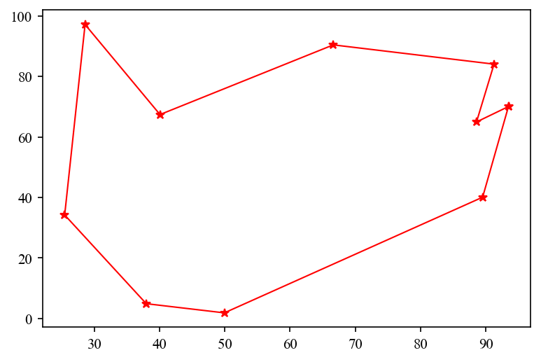

✦ 模拟退火

设置好初始温度、降温参数、最低温度之后即可开始退火。我在这里尝试了2变换法、3变换法、2 3变换法相结合(设置dice骰子随机选择)的模式，最后发现还是2变换法的效果最佳。

# 设置初始参数
T=1
a=0.999

path_opt=path
sum_opt=sum_d
cnt=0
while T>1e-300:
    # dice=rd.randint(1,2)
    # if dice==1:
    m=rd.randint(1,num-2)
    n=rd.randint(m+1,num)
    delta=dist[path[m-1],path[n-1]]+dist[path[m],path[n]]-dist[path[m-1],path[m]]-dist[path[n-1],path[n]]
    # elif dice==2:
    #     m=rd.randint(1,num-3)
    #     n=rd.randint(m+2,num-1)
    #     delta=dist[path[m],path[n-1]]+dist[path[m],path[n+1]]+\
    #       dist[path[n],path[m-1]]+dist[path[n],path[m+1]]-\
    #       dist[path[m],path[m-1]]-dist[path[m],path[m+1]]-\
    #       dist[path[n],path[n-1]]-dist[path[n],path[n+1]]

    if delta<0 or rd.random()<np.exp(-delta/T):
        # if dice==1:
        path[m:n]=path[n-1:m-1:-1]
        # elif dice==2:
        #     path[m],path[n]=path[n],path[m]

        sum_d+=delta
        cnt=0
        if sum_d<sum_opt:
            path_opt=path
            sum_opt=sum_d
    else:
        cnt+=1
        if cnt==300:
            break
    T=a*T

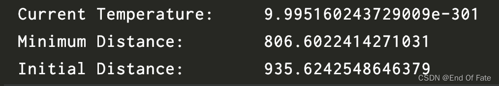
print("Current Temperature:\t",T)
print("Minimum Distance:\t\t",sum_opt)
print("Initial Distance:\t\t",init_sum)
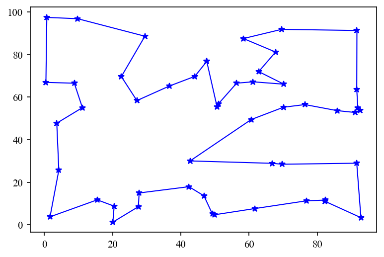
x=loc[path_opt,0]
y=loc[path_opt,1]
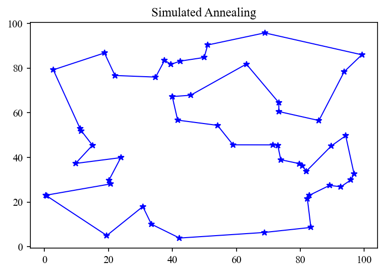
plt.plot(x,y,'b*-',linewidth=1)
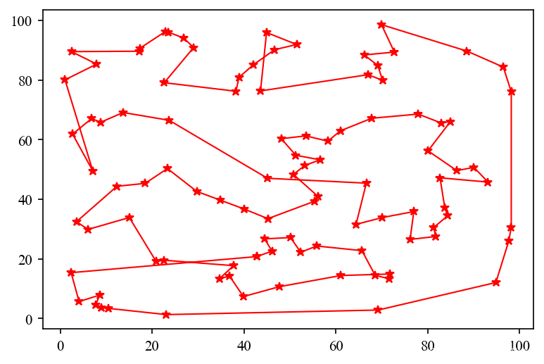
plt.show()

其中一例的结果如下：

顺便将其可视化：

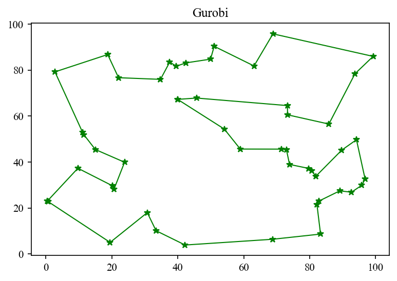
Gurobi

想着用Gurobi也来插一脚，没想到花的时间比码上面的模拟退火还长。因为这里有个问题——如何保证Gurobi给出的解是一个连通图？

仔细想想，会发现多个连通图和一个连通图的总边数以及每个顶点度要求都是相同的，如果优化模型对连通性没有限制的话会出大问题：

后来发现Gurobi官方有给出求解TSP问题的案例，详情戳这。

他在上述模型中又添加了以下约束(*)：

简单地说，如果一个解中包含多个连通分图，那么肯定存在真子集 $S\subset Cities$ ，S中所有的边数(两个端点都在S中)之和==S中的城市数量，且满足这个条件的S即为一个连通分图。因此他就非常暴力地把所有真子集都枚举一遍，让他们都不满足这个条件。

然而在实际实现的过程中，这是个糟糕透顶的想法。因为如此一来约束个数会随着城市数的增加而呈指数式增长。说实在一点，理想是理想，现实是现实。那咋办呢？不要慌，既然Gurobi出了官方文档，说明他们还是有能力解决的。

于是乎他们拿出了名叫Lazy Constraints的法宝，翻译一下应该叫惰性约束，顾名思义，这个约束非常的懒，只有在指定条件才会跳出来判断解的合理性。也就是说，在正常求解的过程中不会添加该约束，在用户指定的情况下再去判断，这样就轻松多啦。

本来想着直接套用官方模版跑一通，奈何他刚开始直接读取了一个json文件，不是很清楚读完后的数据格式，部分地方也没看懂在做什么，导致在套用自己变量后总会出现这样那样的小bug，很烦，简单地重构了下。

想要构造惰性约束需要自己实现一个Callback函数来指定什么条件调用该函数，然后该函数再决定满足什么要求时添加Lazy Constraint：

def delSubtour(model, where):
    # GRB.Callback.MIPSOL：发现新的MIP解
    if where == GRB.Callback.MIPSOL:
        # make a list of edges selected in the solution
        vals = model.cbGetSolution(model._vars)
        edges = gp.tuplelist((i, j) for i, j in model._vars.keys()
                             if vals[i, j] > 0.5)
        adj = {}
        for i, j in edges:
            adj.setdefault(i, set()).add(j)
            adj.setdefault(j, set()).add(i)
        circle = set([0])
        next = set([0])
        new = set()
        while next:
            for k in next:
                new |= adj[k]
            next = new - circle
            circle |= next

        if len(circle) < num:
            model.cbLazy(gp.quicksum(model._vars[i, j] for i, j in combinations(circle, 2)) <= len(circle) - 1)

Callback函数的条件选项可以见官方文档。where指定调用条件，我这里的MIPSOL是指当Gurobi找到一个混合整数规划(MIP)解(SOL)时，就会执行该函数的主体部分。而主体部分先通过cbGetSolution函数获取找到的该解，然后将的顶点元组对放入一个列表中，根据该列表建立一个通过城市编号可以访问连接顶点的邻接字典adj，最后求出0号城市所在连通图的城市个数，与城市总数进行比较就能说明所有城市是否连通。如果不连通，此时再添加约束(*)。

Gurobi求解的完整代码如下：

import gurobipy as gp
from gurobipy import GRB
import numpy as np
import random as rd
# combinations(list,n): 枚举所有长度为n的全排列
from itertools import combinations, product


def delSubtour(model, where):
    # GRB.Callback.MIPSOL：发现新的MIP解
    if where == GRB.Callback.MIPSOL:
        # make a list of edges selected in the solution
        vals = model.cbGetSolution(model._vars)
        edges = gp.tuplelist((i, j) for i, j in model._vars.keys()
                             if vals[i, j] > 0.5)
        adj = {}
        for i, j in edges:
            adj.setdefault(i, set()).add(j)
            adj.setdefault(j, set()).add(i)
        circle = set([0])
        next = set([0])
        new = set()
        while next:
            for k in next:
                new |= adj[k]
            next = new - circle
            circle |= next

        if len(circle) < num:
            model.cbLazy(gp.quicksum(model._vars[i, j] for i, j in combinations(circle, 2)) <= len(circle) - 1)


m = gp.Model("TSP")

vars = m.addVars(dist.keys(), obj=dist, vtype=GRB.BINARY)

# Symmetry
m.addConstrs(vars[j, i] == vars[i, j] for i, j in dist.keys())

# two edges to each city
m.addConstrs((vars.sum(i, '*') == 2) for i in range(num))

# Optimize the model
m._vars = vars
m.Params.lazyConstraints = 1
# setObjective函数此时似乎没用
# m.setObjective(vars.prod(dist), GRB.MINIMIZE)
m.optimize(delSubtour)


vals = m.getAttr('x', vars)
edges = gp.tuplelist((i, j) for i, j in vals.keys() if vals[i, j] > 0.5 and i < j)
adj = {}
for i, j in edges:
    adj.setdefault(i, []).append(j)
    adj.setdefault(j, []).append(i)
isVisited = [False] * num
x = [];
y = []
idx = 0
total = 0
for i in range(num - 1):
    x.append(loc[idx, 0])
    y.append(loc[idx, 1])
    pre = idx
    isVisited[idx] = True
    idx = adj[idx][0] if not isVisited[adj[idx][0]] else adj[idx][1]
    total += dist[pre, idx]

total += dist[idx, 0]
x.append(loc[0, 0])
y.append(loc[0, 1])
print("Minimum Distance：", total)


import matplotlib.pyplot as plt
# 设置字体
plt.rc('font', family='Times New Roman')
# 设置图像的像素
plt.rcParams['figure.dpi'] = 150
# 设置字体的颜色
plt.rcParams['text.color'] = 'black'
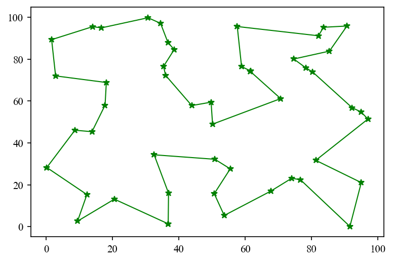
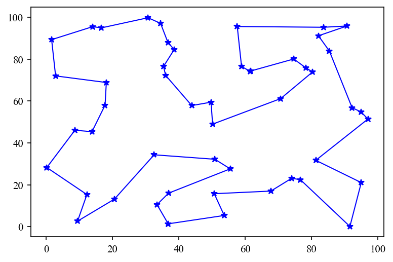
plt.plot(x, y, 'b*-', linewidth=1)
plt.show()

由于Gurobi求解的是最优解，因此规模一旦稍大就要跑很久。城市数量为50左右的求解速度还是很快的，100就开始思考人生了。

逆行的炸酱面

关注

4
点赞
踩
11

收藏

觉得还不错? 一键收藏
0
评论
模拟退火+Gurobi 解决旅行家问题TSP

模拟退火算法，顾名思义，模拟晶体退火过程。晶体在加热后固体化为液态，内部原子运动加剧，会离开原有位置向四周扩散。此时慢慢进行退火冷却使其重新固化，粒子往往会停留在比原先能量低得多的位置上，本质上也是通过随机性跳出局部最优。本文尝试用模拟退火算法对TSP问题(travelling salesman problem)进行求解，并与Gurobi求解器进行对比。
复制链接

扫一扫