Chapter10 : Deep Neural Networks for QSAR

reading notes of《Artificial Intelligence in Drug Design》

---

1.Introduction

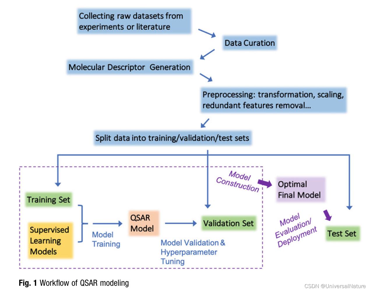
• QSAR models are regression or classification models that predict the biological activities of molecules based on the features derived from their molecular structures.
• QSAR models are developed by training machine learning algorithms that learn the relationships between molecular descriptors and known molecular properties or bioactivities measured in previous experiments.
  
• Cherkasov et al. provided a comprehensive survey of QSAR modeling, which included the historical development of the field and the evolution of its methodology, as well as guidelines for developing reliable QSAR models.
• A more recent review by Muratov et al. focused on modern trends and technological advances in QSAR modeling over the past 5 years and highlighted how methods developed in traditional QSAR areas have been applied to similar fields such as quantum chemistry, materials informatics, nanomaterials informatics, synthetic organic chemistry and polypharmacology.
• In additional to the choice of DNN model architecture and input molecular representations, there are multiple ways to boost the predictive power of a model based on the specific QSAR task it performs and the availability of relevant datasets.

2.Featurization of Molecules

2.1.Feature Vector

• There are many types of chemical descriptors that can be used to characterize a molecule as a list of features.
  • Constitutional descriptors include simple measures of the chemical composition of a molecule, such as its molecules weights, total number of atoms.
  • Topological descriptors are graph invariants (or topological indices) derived from a molecular graph in which atoms are vertices and covalent bonds are edges, such as Wiener index, Extended connectivity fingerprints (ECFPs).
  • Fragment descriptors either note the presence or count the frequency of certain structural fragments in a molecule, such as atom pair (AP) descriptors.
• An encyclopedic guide to molecular descriptors, including the definition, historical development and example usages, is provided by Todeschini et al..
• Different categories of molecular descriptors can be concatenated into a single high-dimensional feature vector to boost the prediction performance of QSAR models.

2.2.Molecular Image

• Two-dimensional drawings of molecular images with red, green, and blue (RGB) channels, created using RDKit, have been used to train convolutional neural networks (CNN). An earlier work by Goh et al. developed CNN model with single-channel gray-scale molecular images as inputs, where discrete values are used to represent atoms or bonds in the two-dimensional molecular structure image. Data augmentation techniques such as random rotation, zooming, and flipping are recommended during the training process for better performance.

2.3.Molecular Graph

• Graphical representations of molecules, where nodes represent atoms and undirected edges represent bonds, can be directly used as inputs for graph convolutional neural networks (GCNs). In addition to the adjacency matrix, which is a description of the connections between atoms, lists of atom and bond features must also be included as an input to GCNs.

2.4.SMILES String

• The simplified molecular-input line-entry system (SMILES) is a chemical notation system that describes molecular structures using strings.
• Because recurrent neural network (RNN) and long short-term memory (LSTM) models have been success- fully used in the field of natural language processing (NLP), which can handle complex text strings, these models have also been used for QSAR modeling with SMILES strings

2.5.Unsupervised Embedding

• Mol2vec is an unsupervised method for learning high-dimensional embeddings of molecular substructures. In the Mol2vec model, molecular substructures derived from the Morgan algorithm are considered “words,” which can then be ordered to represent a molecular “sentence.”

3.Deep Neural Network Architectures

3.1.Multilayer Perception

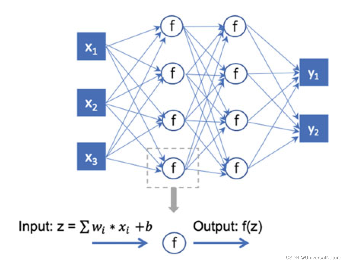
• A practical guide for implementing MLP for QSAR models can be found in Ma et al.

3.2.Convolutional Neural Network

• In contrast with MLP, the CNN model has local connections between adjacent layers instead of fully connected layers, which allows for a much easier training process and better generalization performance for structured input data.
  
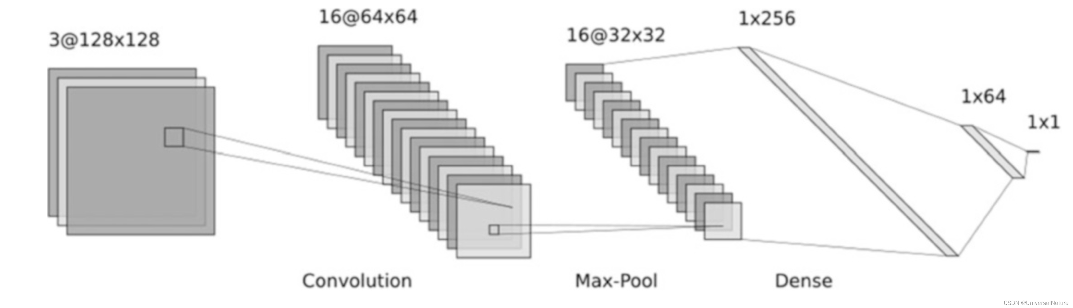
• Many studies have successfully used CNNs to build QSAR models, such as “Chemception” model developed by Goh et al., “DeepNose” model proposed by Tran et al.

3.3.Graph Convolutional Neural Networks

• The first use of GCN architecture in a QSAR model was in the “neural fingerprints” model proposed by Duvenaud et al., who demonstrated that the data-driven neural graph fingerprints generated by GCNs achieve comparable or better predictive performance than ECFPs in a diverse set of QSAR tasks.

3.4.Long Short-Term Memory

• Recurrent neural networks (RNN) are a class of neural networks that were designed for time series or sequential data. Due to their success in language models, LSTMs have been applied in QSAR/QSPR models that learn directly from the SMILES text representations of input molecular structures.

4.Improving Model Performance

4.1.Hyperparameter Optimization

• The cross-validation method is commonly used to select the optimal hyperparameter set according to certain evaluation metrics.
• Manual search and grid search were originally the two most widely used strategies, both techniques require human experts to make various modifications by trial and error or experience.
• Ma et al. helped make DNNs more practical for QSAR modeling in an industrial drug discovery context by providing a set of recommended hyperparameters that lead to consistently good DNNs across a diverse set of QSAR tasks. Their recommended DNN hyperparameters subsequently have served as a baseline architecture for many subsequent works in QSAR modeling.
• Random search and Bayesian optimization are two popular alternatives to the traditional manual search or grid search methods for hyperparameter optimization.
  • In the improved random search strategy, adaptive resource allocation algorithms allocate more resources to promising hyperparameter settings. Empirical studies have demonstrated that this resource allocation algorithm increases search speed by an order of magnitude relative to the original random search approach.
  • The Bayesian optimization search strategy is a sequential model-based optimization (SMBO) approach. In this approach, the algorithm uses an easy-to-evaluate surrogate function to approximate a computationally expensive objective function (such as the performance metrics in DNNs). The search algorithm sequentially proposes the next candidate configurations based on the surrogate model.
  • There are two main components of a Bayesian optimization algorithm: a probabilistic surrogate model of the objective function and an acquisition function that recommends the next candidate point for evaluation.
    • A popular choice of surrogate model is the Gaussian processes (GP).
    • The acquisition functions handle the trade-off between exploration and exploitation.
    • There are several common choices of acquisition function, including the probability of improvement, expected improvement and GP upper confidence bound functions.
    • Snoek et al. provided a practical guide for Bayesian optimization.
• Human knowledge and experience can still be helpful for specifying a narrower search space or a better initialization for these computational algorithms.

4.2.Multitask Learning

• The multitask learning approach aims at improving predictive performance of a DNN by jointly modeling multiple related tasks. In this approach, a shared representation for all tasks is typically learned by training the tasks in parallel.
• This multitask DNN approach for QSAR modeling was originally proposed by the winning team in the Kaggle QSAR competition, who achieved a relative accuracy improvement of approximately 15% relative to the baseline model.
• Although multitask learning has been successfully applied in many QSAR modeling and drug discovery problems, careful consideration is required to determine whether a specific task will benefit from multitask modeling with additional tasks.
• Xu’s results demonstrated that multitask learning is beneficial when the molecular activities are correlated between tasks, and that structurally similar molecules could help share information across targets.
• There are two general types of multitask learning approaches in deep neural networks: hard parameter sharing and soft parameter sharing:
  • In hard parameter sharing, the neural network structure is composed of hidden layers that are shared across different tasks, followed by several task-specific hidden layers and/or an output layer. The multi-output neural nets described above is a special case of hard parameter sharing.
  • In soft parameter sharing, hidden layers are not shared across tasks; instead, the network uses feature-sharing mechanisms such as regularization and ensembling, while the model for each task maintains its own parameters.
• In addition to these novel network structures, various other optimization methods could be adopted to improve the training efficiency of multitask neural nets:
  • Kendall et al. demonstrated that the choice of multitask loss function is critically important for task-dependent uncertainty.
  • Chen et al. designed an alternative gradient normalization algorithm that dynamically adjusts the gradient magnitudes and balances the training rates of different tasks.

4.3.Transfer Learning

• Transfer learning is classified into three subcategories based on the relationships between the source and target domains and tasks: inductive transfer learning, transductive transfer learning, and unsupervised transfer learning. The first two subcategories are more commonly used in QSAR:
  • Inductive transfer learning: In this model, the source tasks and the target task are different, regardless of whether they have the same domains. For example, the measured activities of the source and target tasks are different, even though they may share a common subset of molecules. This case is analogous to the examples provided in the multitask modeling section, except here we only care about the model performance for target task.
  • Transductive transfer learning: Here, the source and target tasks are the same, but the domains are different. For example, the same molecular activity is measured in multiple data sets but with different distributions of molecular structures. In machine learning, this situation is also called “covariate shift” or “dataset shift”。
• In general, four typical types of knowledge are transferred from source tasks to the target task: training data instances, feature representation, model parameters, and relational knowledge.
• A comprehensive overview of the various transfer learning methodologies and their applications to data mining is provided by Pan et al.
• A more recent review by Simoes et al. discusses transfer learning techniques in the context of QSAR modeling and presents potential applications of transfer learning in medicinal chemistry studies.
• Cai et al. reviewed state-of-the-art applications of transfer learning for drug discovery, focusing primarily on DNN-based algorithms.
• Li et al. adopted a multistage transfer learning approach developed in NLP for molecular property/activity prediction.
• Goh et al. developed a transfer learning approach that used weak supervised learning to integrate rule-based knowledge from previous chemical feature engineering research into DNNs.
• Iovanac et al. developed a novel feature representation transfer approach in which an autoencoder neural network was used to create a latent space as the shared feature in transfer learning.
• A critical first step in transfer learning is using expert experience to select compatible source datasets, as knowledge from unrelated source datasets may result in “negative transfer,” which hurts the model generalization performance for the target task.
• As an alternative to relying on experiment experience, data-driven methods have been designed to circumvent negative transfer. For exam- ple, Hu et al. developed a pretraining strategy for Graph Neural Networks (GNNs) that effectively avoided negative transfer for downstream target tasks. The key idea behind their approach, which is applicable to various GNN architectures, was performing both node-level and graph-level pretraining.

5.Model Interpretation

5.1.Uncertainty Estimation

• Conformal prediction is a model-agnostic approach for quantifying confidence in model predictions and is applicable to both regression and classification tasks.
• Given the size of the training data in most QSAR problems, the computationally efficient inductive conformal prediction (ICP) framework is suitable for conformal prediction. The general steps of ICP are:
  • Specify a supervised learning algorithm (either regression or classification) as the underlying learning method.
  • Define a nonconformity measure to quantify how unusual a sample is compared to the rest of samples. For example, the nonconformity can be defined as the absolute value of residuals for regression problems or, for classification problems, as one minus the predicted probability of a sample belonging to a given class (also called the “least confidence score”).
  • Divide the available training data into a “proper training set” and a “calibration set.”
  • Use the proper training set for model fitting and then apply the trained model to the calibration set. Calculate the nonconformity score αj for each calibration set sample x_j (0<j<n+1).
  • Given a new sample x_n+1 in the test set and a possible label Y of this new sample, calculate the nonconformity score for x_n+1 and compare it to the nonconformity scores of the calibration set samples. Compute a p-value for x_n+1 by calculating the fraction of samples with larger nonconformity scores: p n + 1 Y = # { j = 1 , . . . , n + 1 : a j > a n + 1 } n + 1 p_{n+1}^Y=\frac{\#\{j=1,...,n+1:a_{j}>a_{n+1}\}}{n+1} pn+1Y​=n+1#{j=1,...,n+1:aj​>an+1​}​
  • For a specified significance level $ϵ\in (0,1)$, which corresponds
    to a confidence level of $1-ϵ$, the prediction region for x_n+1 contains the set of all possible labels Y with a p-value larger than the significance level: ϝ n + 1 ϵ = { Y : p n + 1 Y > ϵ } \digamma^{\epsilon}_{n+1}=\{Y:p_{n+1}^Y>\epsilon\} ϝn+1ϵ​={Y:pn+1Y​>ϵ}.
• This flexible framework has been extensively applied to QSAR models built with a variety of supervised learning algorithms.
  • Cortes-Ciriano et al. proposed the “deep confidence” method for estimating uncertainty, which integrates conformal prediction with DNNs to generate valid and efficient prediction intervals for QSAR regression tasks. The “deep confidence” method requires a “snapshot ensemble” of DNN models. This snapshot ensemble is created by saving model weights periodically while training a single DNN, such that the ensemble of DNNs consists of multiple snapshots of the optimization path.
  • Another uncertainty estimation technique, called the “dropout conformal predictors” approach, uses test-time dropout instead of the snapshot ensemble to create a DNN ensemble model. It achieved comparable validity and efficiency with less model storage effort than the “deep confidence” method.
• Another major category of uncertainty estimation methods uses a probabilistic approach, in which the posterior distribution of model outputs is explicitly modele.
  • One such probabilistic approach is the mean-variance estimation (MVE) method, which modifies the output layer of a neural network to predict both the mean and variance of the target property and uses negative Gaussian log-likelihood loss for model training.
  • Khosravi et al. evaluated several probabilistic techniques for constructing prediction intervals (PIs) for neural nets, including the delta, Bayesian, bootstrap, and MVE methods. Their results suggested that the delta and Bayesian methods yield high-quality and reproducible PIs, whereas the MVE and bootstrap methods require a lower computational cost and produce PIs that are more variable in length.
  • Based on comparisons of both regression accuracy and uncertainty quantification accuracy across several QSAR regression models, Hirschfeld et al. recommended a union-based method that combines MPNN and RF.
• Based on previous explorations, the choice of uncertainty estimation technique should depend on the goal of the analysis, the computational costs, the characteristic of the given QSAR task, and the desired properties of the resulting PIs.

5.2.Feature Importance

• There are three main categories of feature importance techniques: perturbation-based methods, gradient-based methods, and the surrogate-model approach:
  • Perturbation-based methods assess feature importance by determining how much model performance decreases when certain input features are modified, masked, or deleted.
    • One such method is the permutation-based variable importance (VI) measure proposed by Breiman, which was originally designed for RF models and has been adapted to neural network-based QSAR models.
    • The “RISE” algorithm by Petsiuk et al. is another perturbation-based method and was designed for any black-box model that produces a scalar confidence score, such as a neural network classifier that predicts the probability of being in a certain class.
    • One advantage of these model-agnostic perturbation-based methods is that they are easy to implement, without requiring any internal weights/gradients or extra modeling effort; however, they suffer from high computational costs when the dimensions of the input features are large.
  • Gradient-based methods compute the partial derivatives of the response (or activation values) with respect to the input variables (i.e.,$\frac{\partial f(x_1,x_2,...,x_n)}{\partial x_i}).$ These partial derivatives effectively measure how much change in the response $f(x_1,x_2,...,x_n)$ is driven by a small change in the input feature $x_i$ around the local neighborhood.
    • Several gradient-based algorithms have been developed to gain a better understanding of the contributions of input features in DNNs; these algorithms include the saliency maps,deconvolutional network, class activation mapping (CAM), Grad-CAM, DeepLift , layer-wise relevance propagation (LRP), and SmoothGrad.
    • The Integrated Gradient method proposed by Sundararajan et al. attributed the model prediction $F(x)$ to each input variable $x_i$ using the path integral of the partial gradient $\frac{\partial f(x)}{\partial x_i}$ along the linear path from a certain baseline $x^{\prime }$ to the input x (i.e., $a_i=(x_i-x_i^{\prime }){\int }_{t=0}^1\frac{\partial f(x^{\prime }+t(x-x^{\prime })}{\partial x_i}dt$, the magnitude of $a_i$ can be interpreted as the contribution from each feature $x_i$. This integrated gradient method has been applied to a GCN network model for QSAR classification tasks.
    • Sanchez-Lengeling et al. evaluated several commonly used feature attribution methods, including SmoothGrad, CAM, Grad-CAM, and Integrated Gradient, across different graph neural net architectures. Their benchmarking results on synthetic molecular datasets with hypothesized binding mechanisms suggested that CAM and Integrated Gradient usually achieve better performance.
    • However, despite of the popularity of gradient-based feature importance methods, the robustness of interpretation against perturbations still remains a challenge.
  • The surrogate-model approach quantifies feature importance using a more interpretable surrogate model that approximates the original black-box prediction model.
  • For example, the Local Interpretable Model-agnostic Explanations (LIME) method was designed to learn interpretable models that are locally faithful to any given model.
  • Like perturbation-based methods, the surrogate model approach is also computationally expensive due to the high-dimensional input space in common QSAR datasets. In addition, the local region explored by the surrogate model may be a “flat” region of the predictor, and thus the sensitivity of the results is not guaranteed.
• More examples of how atom and fragment contributions have been analyzed in QSAR models can be found in the perspective article by Polishchuk.

6.Summary

• The quest to develop highly accurate and broadly interpretable QSAR models has attracted increasing attention in recent years.
• “Domain applicability” is another important issue in the prospective application of QSAR models. This issue is also known as the “dataset shift” problem and is caused by different joint distributions of the inputs and outputs between the training and test sets. Well-calibrated uncertainty estimates are one method for avoiding these unreliable extrapolations. Alternatively, domain adaption methods, such as the adversarial discriminative domain adaptation method, could increase the generalizability of a model by learning deep neural transformations that map both domains into a common feature space.