Chapter18: Machine Learning from Omics Data

reading notes of《Artificial Intelligence in Drug Design》

---

1.Introduction

• Given a number of biological samples N, an omics technology measures a certain number of molecular entities P. Any person familiar with machine learning will immediately recognize this as a feature matrix M ∈ N x P. Usually, P is in the range of a few hundreds up to several thousand features.
• Throughout this chapter, I will use a recently published subset of the LINCS L1000 dataset to illustrate characteristics and pitfalls of omics datasets.
• The aforementioned dataset contains 6000 transcriptome profiles of 640 different compounds distributed over various cell lines, doses, and treatment durations. 3568 samples are classified as DILI positive and 2432 as DILI negative.
• Since the costs of full RNA sequencing for all samples would have been prohibitive, the authors selected 978 representative landmark genes for quantification. This targeted approach (called L1000) is much cheaper and thus allows the profiling of thousands of samples.
• More precisely, all examples make use of the Level 5 data (moderated Z-scores) as features for the machine learning model.
• The code to reproduce the results is available.

2.Data Exploration

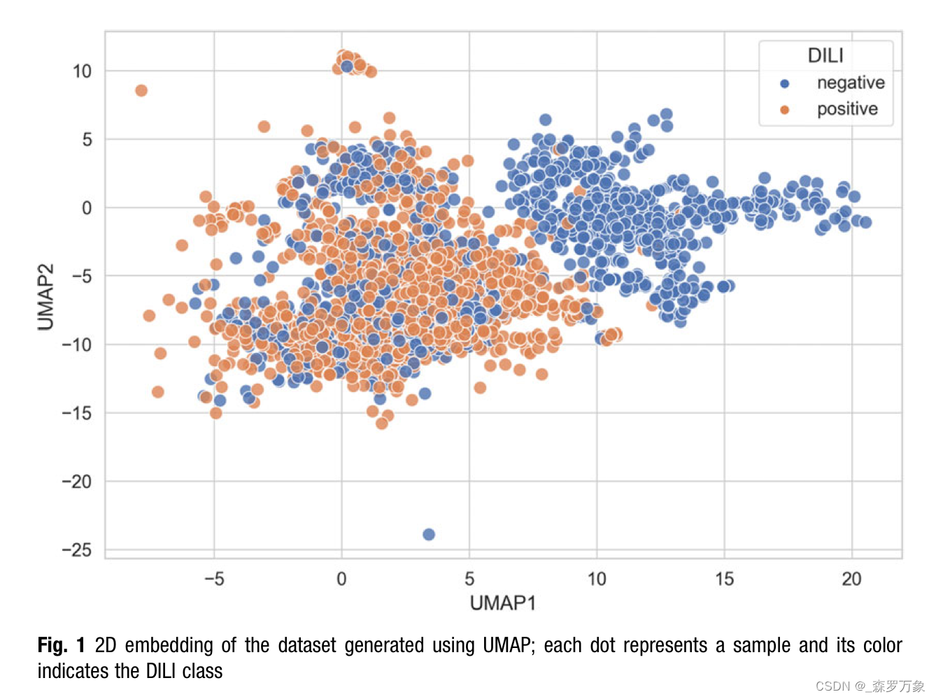
• One way to identify the most obvious outliers and batch effects is to project the data to two dimensions using a dimension reduction method and inspect the scatter plot.
• Figure 1 shows a 2D embedding of the example data generated with UMAP in densMAP mode.
  
• These strongly correlated features add little information, may cause problems when estimating coefficients for linear models, and complicate model interpretation. Thus, it is advisable to either combine them into one feature (e.g., by averaging) or to choose one representative and remove the others. The histogram on the left hand side of Fig. 2 displays the distribution of the maximum absolute Spearman’s correlation for all features.
  
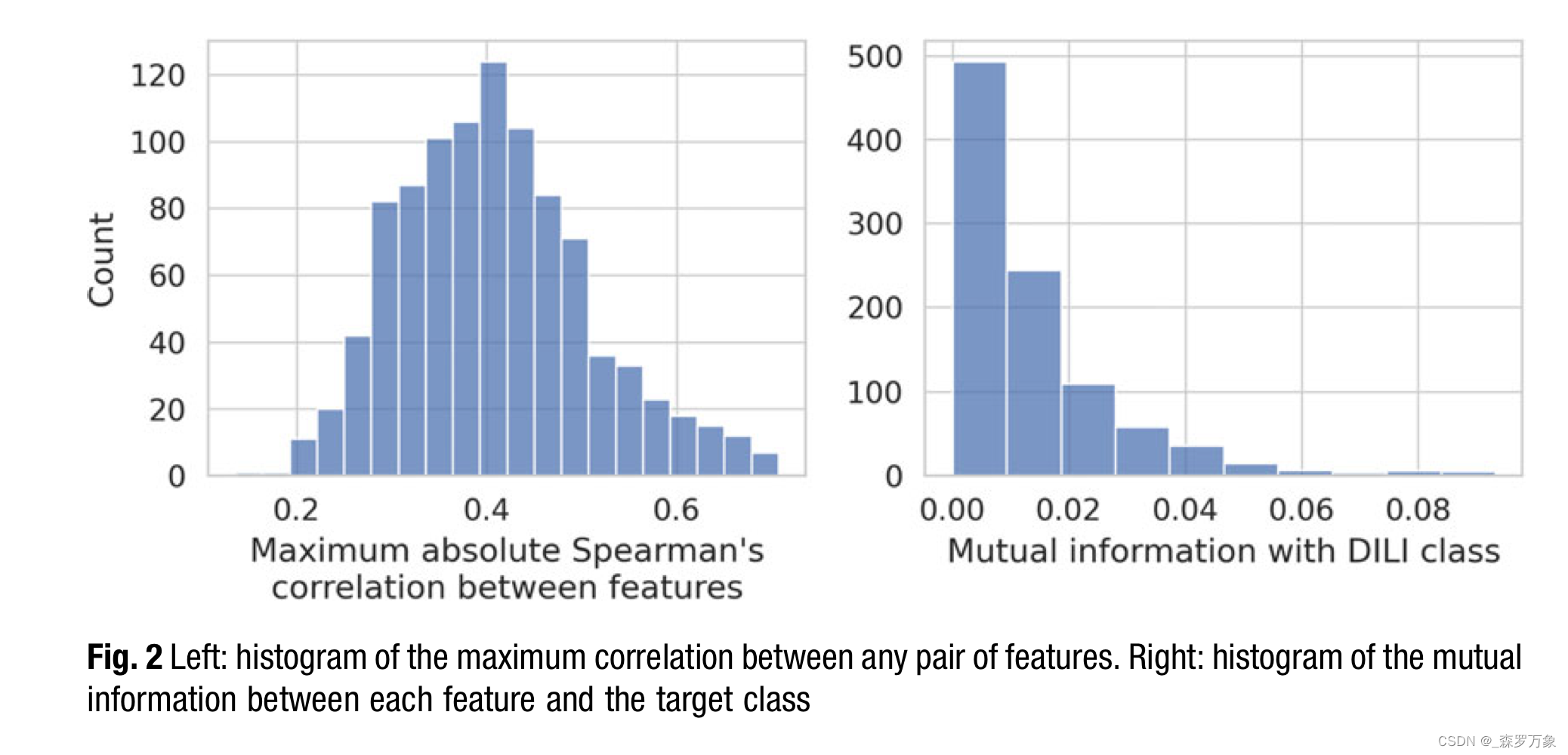
• The right part of Fig. 2 shows a histogram summarizing the mutual information (MI) between each feature and the target, which is the DILI class here. I opted for mutual information as univariate measure because it also captures partial and nonlinear relationships.
• While all scores are far lower than the maximum possible score of 0.67 (the MI between the target vector and itself), there are clearly many uninformative features and very few informative ones. This implies that some kind of feature selection should be part of the machine learning model.

3.Model Defintion

• Building upon the knowledge gathered in the data exploration step, I propose to use a short pipeline implemented using Python 3 and scikit-learn as machine learning model . It consists of three steps: (1) feature standardization, (2) feature selection, and (3) a support vector machine (SVM) as classifier.
  • The SVM assumes that all features are roughly distributed like a standard Gaussian with to zero mean and unit variance. This is not the case for the example data. Therefore, the first step in the pipeline is to standardize all features.
  • As noted in the introduction, obtaining a large number of samples is rather costly and thus we often end up in the N << P regime when dealing with omics data. Here looms the infamous “curse of dimensionality”. Hence, we need to take extra care not to overfit our machine learning models. Regularization and feature selection are the most popular tools to achieve this.

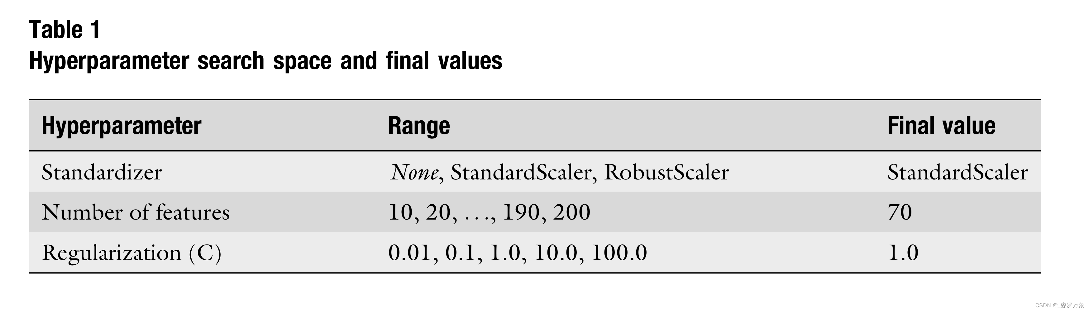
4.Hyperparmeter Search

• Here, I use a simple grid search to find the best values for the hyperparameters. Since the model is fast to train and the number of hyperparameters is low, this is still computationally feasible. However, complex models with many hyperparameters may call for more sophisticated search strategies like Hyperband or Bayesian methods.

5.Model Validation

• Hence, I repeated the complete example using a compound-based split for the validation set and a fivefold cross-validation splitting by compounds for the hyperparameter search.Results indicates that the model does not generalize well to yet unseen compounds and the previously results were achieved because the model memorizes the individual compound signatures.
• If a project comes to this point, I advise to take a step back and reconsider a few things. Is the dataset suitable to address the original problem statement? Is it possible to obtain more or better data? Are other modeling approaches more promising? Does the scope of the project need to be redefined? Maybe it is even best to scrap the project, start over, and work on some other problem.

6.Training of the Final Model and Interpretation

• we assume that we are satisfied with the metrics of our model. The next steps are to train the final model and understand what drives the classifications of the model.
• To generate a model that is ready for use in production, we need to train the pipeline one final time using the best parameters found by the hyperparameter search. This time, we use all the data including training, test, and validation sets.
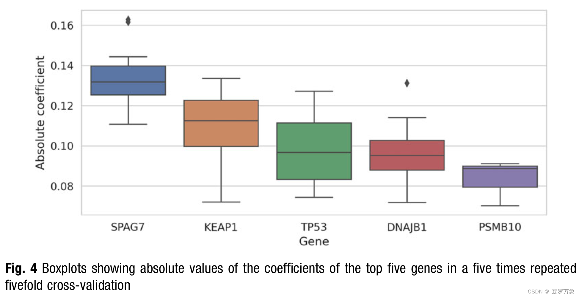
• In theory, we could even determine the class the feature is driving the classification to from the signs of the coefficients. However, as the feature values can be negative, it is a bit more involved to interpret the signs and thus I use the absolute coefficients to display overall relevance in Fig. 4.