


大家好,这一次我们来分享一下有关做10X空间转录组的分析软件SPATA,其实关于10X空间转录组做轨迹分析的文章之前分享过一个,文章在10X空间转录组的轨迹分析,其中用到的软件是stlearn,我们放一张stlearn分析出来的图
今天我们来分享另外一个软件,SPATA,文章在Inferring spatially transient gene expression pattern from spatial transcriptomic studies,我们还是先分享文献,最后分享示例代码。
Abstract
Spatial transcriptomic is a technology to provide deep transcriptomic profiling by preserving the spatial organization.(这个老生常谈了)。Here, we present a framework for SPAtial Transcriptomic Analysis (SPATA, https://themilolab.github.io/SPATA), to provide a comprehensive characterization of spatially resolved gene expression, regional adaptation of transcriptional programs and transient dynamics along spatial trajectories.(运用这个软件来做空间轨迹分析,讲道理,我很好奇!!)。
Brief Communication(这个地方我们总结一下)
Deep transcriptional profiling of single cells by RNA-sequencing maps the cellular composition of tissue specimens regarding cellular origin, developmental trajectories and transcriptional programs(这是单细胞的优势),However, information determining the spatial arrangement of specific cell types or transcriptional programs are lacking and thus can only be predicted indirectly(空间信息的缺失),which is a considerable drawback of this method.(也是众所周知的缺点)。空间组织结构传统的方式是用成像技术提供高精度的信息,但是同时检测的基因和蛋白的数量非常少,当然,已经有了一些新的空间组织检测技术,但受到空间分布细胞精度和深度的制约,Further, data integration, visualization and analysis of transcriptomic and spatial information remains challenging. Here, we present a software tool to provide a framework for integration of high-dimensional transcriptional data within a spatial context.这个软件集友好的可视化界面,分割或轨迹分析,提供了广泛了不同分析方法,In particular, we focus on transient changes of gene expression and aim to infer transcriptional programs that are dynamically regulated as a function of spatial organization.(这个软件就是专门为10X空间转录组做准备的)。
In order to present an overview of possible analytic capabilities of the SPATA workflow,
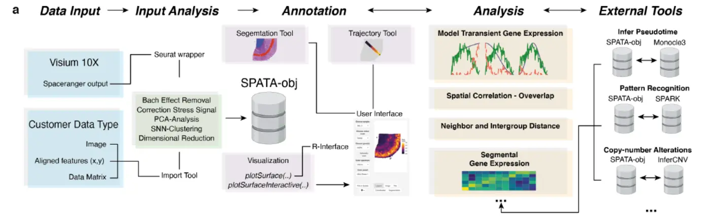
generated spatial transcriptomic datasets from human cortex and human glioblastoma samples using the Visium technology (10X Genomics). The human cortex is separated into defined layers containing different types of neurons and cellular architecture(空间转录组数据是事先注释好的),
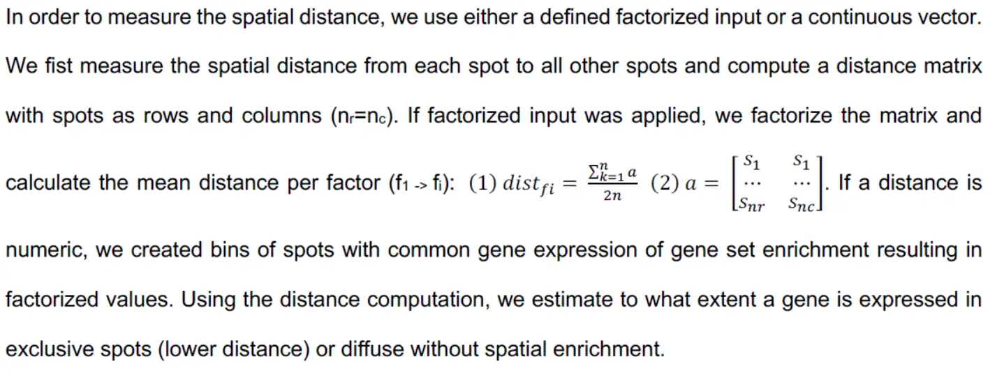
- In a first step, we combine shared-nearest neighbor clustering and spatial pattern recognition by an external tool(SPARK)in order to determine genes with a defined spatially resolved expression pattern.(这个地方类似于Seurat计算空间差异基因)。We found that the cortical layering is accurately reflected by our clustering approach(这个很自然)。In order to gain insights into the spatial organization we provided a tool to compute the spatial distance within the defined layers or correspondent clusters. An increasing distance within individual clusters allows to differentiate between narrowly related or a widespread dispersion of spots within the cluster.(计算空间距离,这个在我分享的文章空间转录组细胞类型的距离分析之二---代码实现,提到过,只不过注意,这里计算的是cluster内部的距离)。
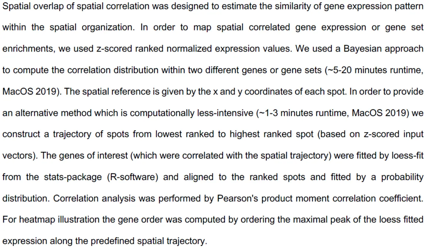
- Next, the spatial overlap of transcriptional programs or gene expression was analyzed using a Bayesian approach(有关贝叶斯的知识大家可以参考我的文章贝叶斯分类器(10X单细胞和10X空间转录组的基础算法)),resulting in an estimated correlation which quantifies the identical arrangement of expression in space.
- In a further step, we aimed to analyze dynamic changes, which were annotated using pseudotime estimation or RNA-velocity.(轨迹推断)。We directly implemented the pseudotime inference from the monocle3 package, but also allow the integration of any other tool such as “latent-time” extracted from RNA-velocity (scVelo). (看来这个软件的轨迹推断需要借助单细胞的轨迹分析软件)。Another option for dynamic gene expression analysis is the detection of defined transcriptional programs along a defined trajectory.(基因的动态表达)。我们在方法中重点关注一下这个。
- Moreover, we provide the opportunity to screen for gene expression or transcriptional programs which transiently change along predefined trajectories by modelling gene expression changes in accordance to various biologically relevant behaviors.(轨迹分析的转变基因)。
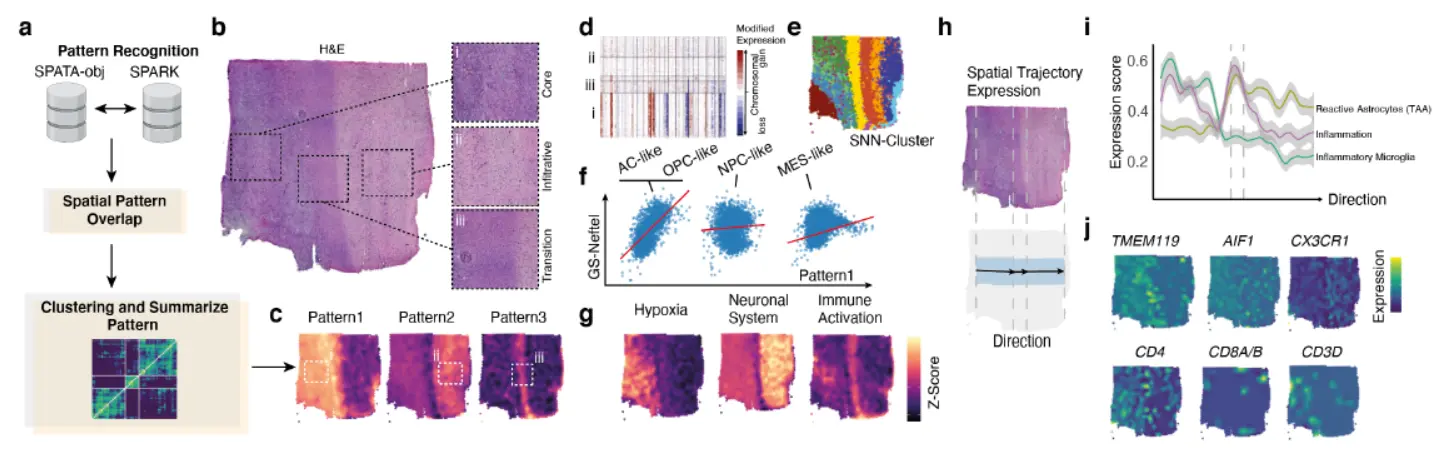
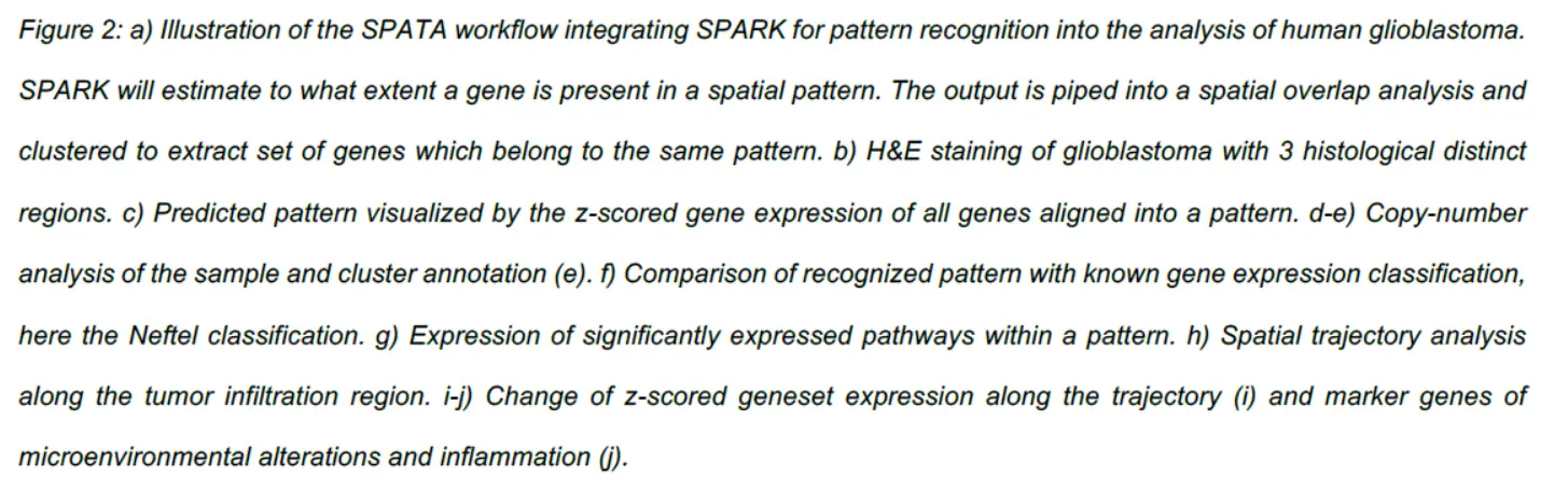
这个地方我们稍微讨论一下 - 第一步,SPARK识别空间pattern,这个pattern需要人为指定,看来这个划分了3个pattern
- 第二步,各个pattern在空间上的映射,这个地方主要对各个pattern做一下富集,看看区域分布
- 第三步,Copy-number analysis of the sample and cluster annotation(空间注释)
- 第四步,Comparison of recognized pattern with known gene expression classification (识别模式与已知基因表达分类的比较 ,看看是否一致)
- 第五步,模式中显着表达的途径的表达(就是显著富集的通路)
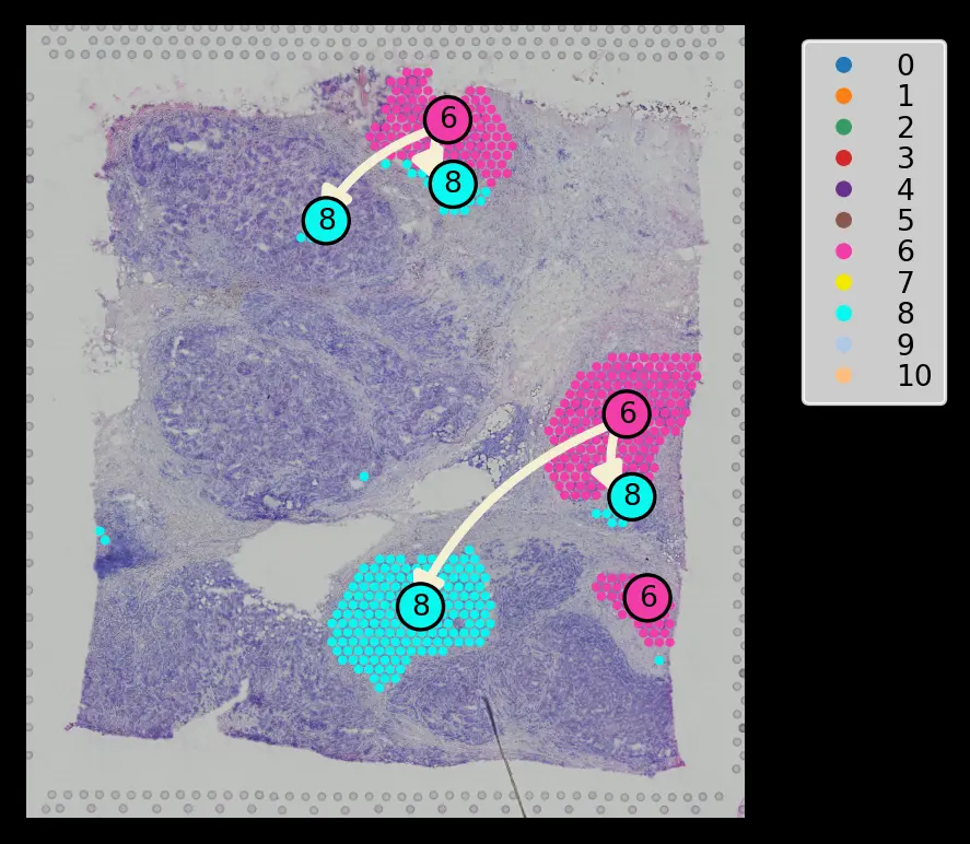
- 第六步,肿瘤区域的空间轨迹分析。
- 第七步,也是最为重要的一步,Change of z-scored geneset expression along the trajectory (i) and marker genes of microenvironmental alterations and inflammation(关键基因的变化)。
看来对空间上的动态变化基因还是要引起重视。不过这里空间SPOT做inferCNV有待商榷。
还有一个很有意思的地方,Thus, we were able to show 116 that immune related genes from myeloid cells and reactive astrocytes were localized in a “glial-scars” resembling structure, sharply separating normal brain from tumor regions Figure 2h. We observed a transient increase of macrophage and microglia activation directed towards the tumor boarder,这个方法是不是值得一试呢?。
Methods,我们关注一下其中的重点
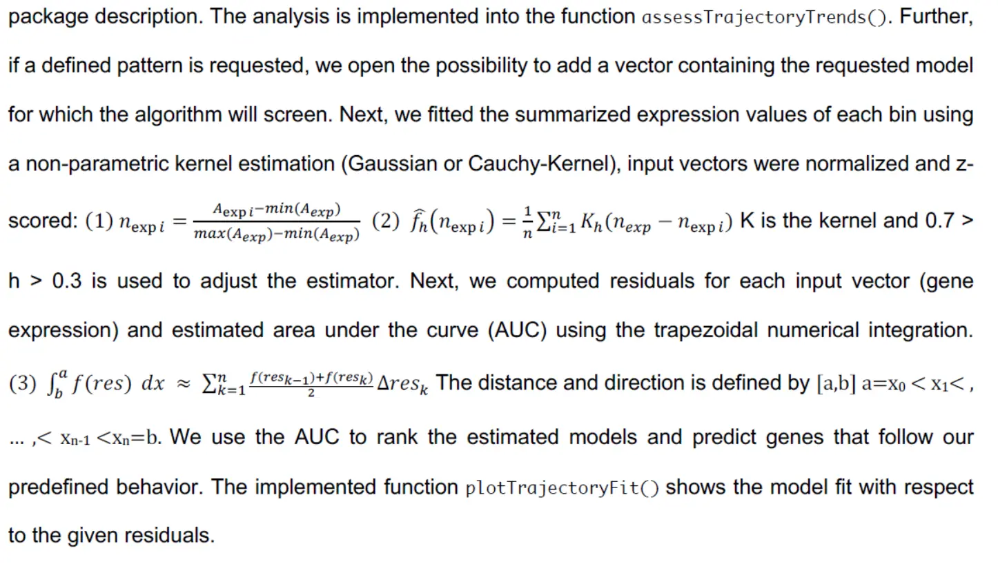
Modeling of transient gene expression along spatial trajectories
Spatial distance measurement
Spatial overlap and correlation analysis
我们来分享一下示例代码
这里的示例代码很多,我们关注一下轨迹部分的代码
Vsiualization
Spatial trajectories
Segmentation
DE - Analysis
空间轨迹推断
With spatial trajectory analysis SPATA introduces a new approach to find, analyze and visualize differently expressed genes and gene-sets in a spatial context. While the classic differential gene expression analyzes this differences between experimental groups as a whole it neglects changes of expression levels that can only be seen while maintaining the spatial dimensions. Spatial trajectories allow to answer questions that include such a spatial component. E.g.:
- In how far do expression levels change the more we move towards a region of interest?
- Which genes follow the same pattern along these paths?
The spatial trajectory tools provided in SPATA enable new ways of visualization as well as new possibilities to screen for genes, gene-sets and patterns of interest.
load package
[library](https://rdrr.io/r/base/library.html)(SPATA)
[library](https://rdrr.io/r/base/library.html)(magrittr)
[library](https://rdrr.io/r/base/library.html)(ggplot2)
[library](https://rdrr.io/r/base/library.html)(patchwork)
load spata-object
spata_obj <- [loadSpataObject](https://themilolab.github.io/SPATA/reference/loadSpataObject.html)(input_path = "data/spata-obj-trajectory-analysis-tumor-example.RDS")
Draw trajectories
Spatial trajectories of a sample in a given spata-object can be drawn interactively using the function createTrajectories() as shown in the example below. createTrajectories() opens a mini-shiny application. This app allows one the one hand to investigate the sample with regards to spatial gene expression like plotSurfaceInteractive() does and on the other hand to draw trajectories through the areas of interest in four easy steps.
library(SPATA)
# open interactive application
spata_obj <- [createTrajectories](https://themilolab.github.io/SPATA/reference/createTrajectories.html)(object = spata_obj)
1. Drawing
Draw the trajectory interactively by clicking on the locations where you want the start and endpoints to be. If you click more than two times the trajectory is divided into sub-trajectory parts which will be displayed by subsequent plotting functions. Hence, it makes sense to stop everytime where you would expect a change as this will be highlighted by the transition from part to the subsequent one.
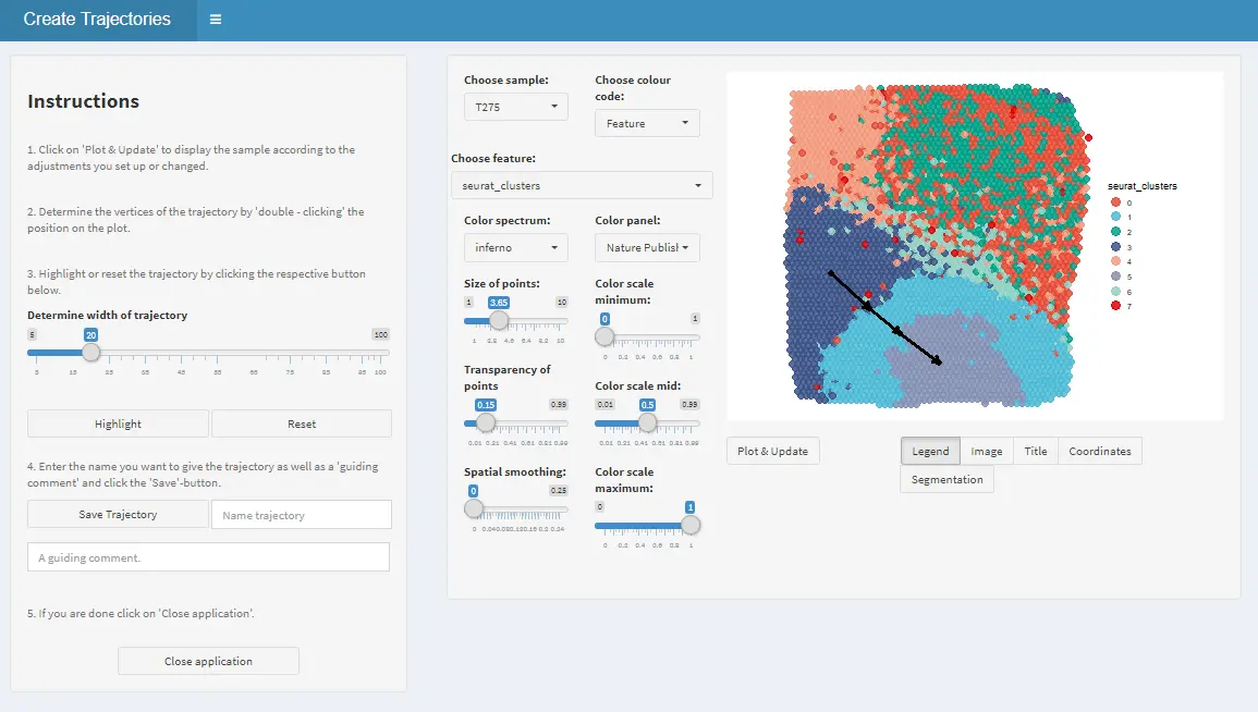
2. Highlighting
If start- and end-points are set adjust the trajectory width to and click on ‘Highlight’.
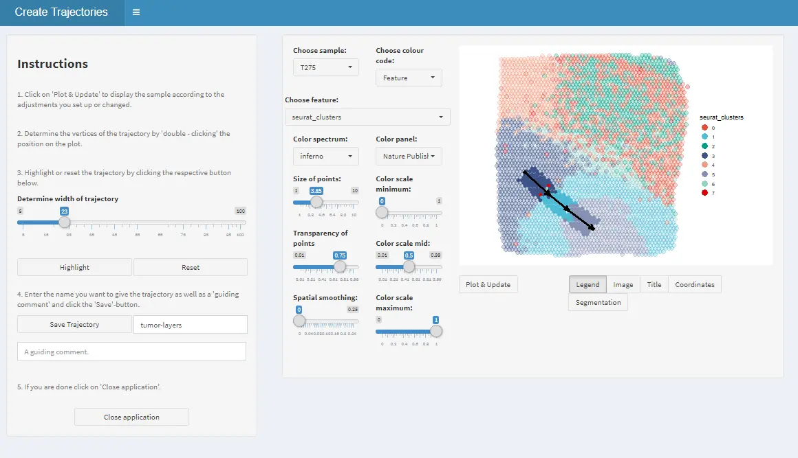
3. Naming
If you are satisfied with your trajectory enter a valid trajectory name and - if you want - a comment.
4. Saving
Click on ‘Save’ and on ‘Close application’ in order to return the updated spata-object.
Trajectories are stored inside the object itself. Therefore createTrajectories() returns an updated version of the object that was specified as the function’s input now containing the additional trajectories.
To obtain all trajectory names that have been drawn and saved in your spata-object use getTrajectoryNames(). Depending on the number of samples specified it returns a character vector or a list of such.
get trajectory names
getTrajectoryNames(object = spata_obj)
## [1] "tumor-layers"
Visualize trajectories
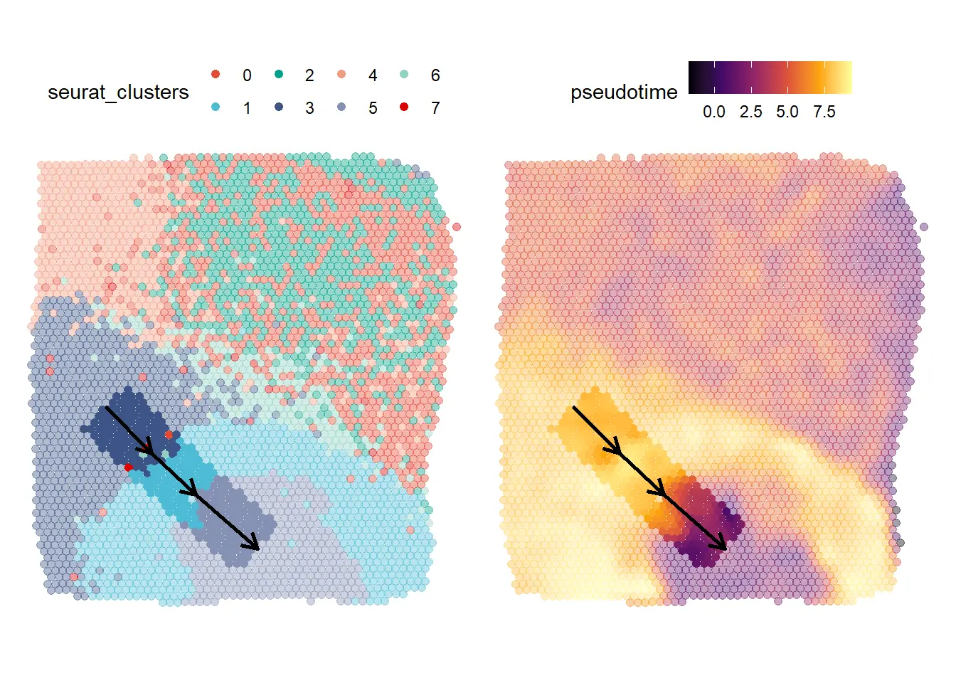
In order to visualize specific trajectories make use of plotTrajectory().
plotTrajectory(object = spata_obj,
               trajectory_name = "tumor-layers",
               color_to = "seurat_clusters",
               pt_size = 1.7,
               pt_clrp = "npg",
               display_image = FALSE) +
               theme(legend.position = "top") +

plotTrajectory(object = spata_obj,
               trajectory_name = "tumor-layers",
               color_to = "pseudotime",
               pt_size = 1.7,
               smooth = TRUE,
               smooth_span = 0.0125,
               display_image = FALSE) +
               theme(legend.position = "top")
Visualize trajectory trends
Trajectory trends via lineplots
To display the trend of certain variables along a trajectory via lineplots use one of the following three functions:
A call to one of those three functions will return a smoothed lineplot where the direction of the trajectory is mapped onto the x-axis and the values of the chosen aspects are mapped onto the y-axis. All functions follow the same concept and share the majority of their arguments. Still, they feature slight differences given the nature of their aspects to display.
The following three arguments have to be set in order to specify the trajectory that is to be analyzed:
- object
- trajectory_name
- of_sample (if more than one sample exists in the object, else it can be neglected)
The way values are smoothed and displayed can be manipulated via:
- smooth_method
- smooth_span
- smooth_se
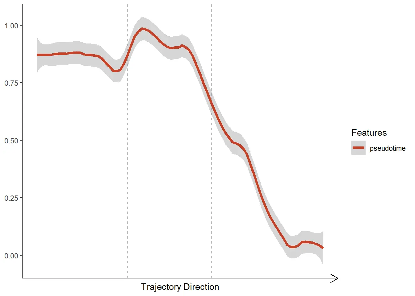
Features along trajectories
Specify the features of interest via the argument features. Note that the function will compute the mean of all points on the axis orthogonal to the trajectory’s direction. As only numeric variables allow for such computation displaying the trend of categorical variables (e.g. cluster) is not possible via lineplots.
plotTrajectoryFeatures(object = spata_obj,
                       trajectory_name = "tumor-layers",
                       features = "pseudotime",
                       smooth_method = "loess",
                       smooth_span = 0.2,
                       smooth_se = TRUE)</pre>
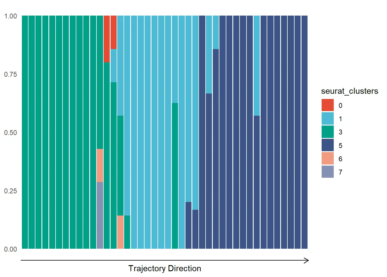
In order to plot discrete features use `plotTrajectoryFeaturesDiscrete().
plotTrajectoryFeaturesDiscrete(object = spata_obj,
                               trajectory_name = "tumor-layers",
                               discrete_feature = "seurat_clusters",
                               clrp = "npg",
                               display_trajectory_parts = FALSE)
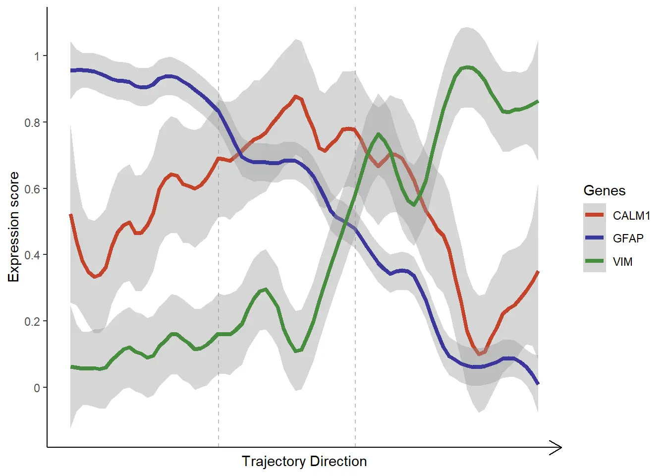
Genes and gene-sets along trajectories
Specify the genes or gene-sets of interest by using the respective functions and arguments.
# gene-set names
genes_of_interest <- [c](https://rdrr.io/r/base/c.html)("CALM1", "VIM", "GFAP")

# plot lineplot
plotTrajectoryGenes(object = spata_obj,
                    trajectory_name = "tumor-layers",
                    genes = genes_of_interest,
                    smooth_span = 0.2,
                    smooth_se = TRUE)
plotTrajectoryGeneSets(
  object = spata_obj,
  trajectory_name = "tumor-layers",
  gene_sets = "HM_HYPOXIA",
  display_trajectory_parts = FALSE) + # results in missing vertical lines
  ggplot2::theme(legend.position = "top")

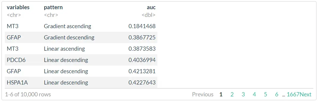
Analyze & model trajectories
To find variables that follow a certain trend along the trajectory of interest use assessTrajectoryTrends(). It fits the trajectory-trends of all specified variables to a variety of patterns and assesses their fit by calculating the area under the curve of the residuals.
all_genes <- getGenes(spata_obj)
all_gene_sets <- getGeneSets(spata_obj)

# obtain an assessed trajectory data.frame for all genes
atdf_gs <- assessTrajectoryTrends(object = spata_obj,
                                  trajectory_name = "tumor-layers",
                                  variables = all_genes)

# obtain an assessed trajectory data.frame for all gene-sets
atdf_gene_sets <- assessTrajectoryTrends(object = spata_obj,
                                         trajectory_name = "tumor-layers",
                                         variables = all_gene-sets)

# output example
atdf_gs
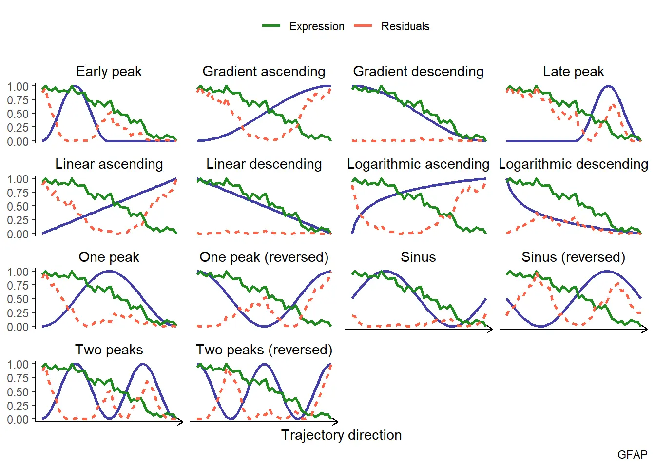
The resulting data.frame contains the evaluation of all fits for all provided variables. plotTrajectoryFit() visualizes the fitting results for a particular variable.
# compare the trend of a variable to different models
plotTrajectoryFit(object = spata_obj,
                  trajectory_name = "tumor-layers",
                  variable = "GFAP",
                  display_residuals = TRUE) +
  ggplot2::theme(legend.position = "top")
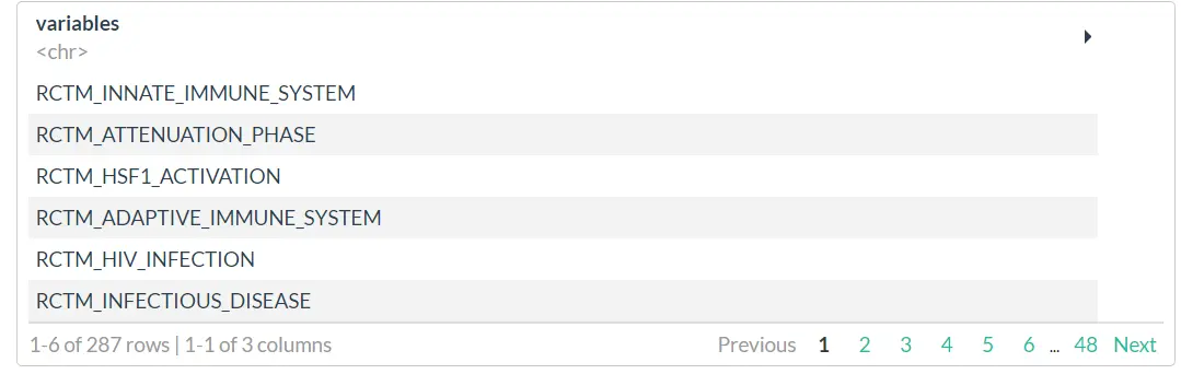
To get a summary of your trajectory assessment use examineTrajectoryAssessment() which displays the distribution of all areas under the curve measured. Use filterTrend() or a combination of dplyr::filter() and dplyr::pull() on your assessed trajectory data.frame in order to extract the variables following a specific trend to a certain quality-degree.
# example 1: extract all variables that follow the linear descending trend while moving towards the hypoxic area (See Figure 2.1)
# with an auc-evaluation equal to or lower than 2
descending_gene_sets <-
  filterTrends(atdf = atdf_gene_sets,
               limit = 2,
               trends = [c](https://rdrr.io/r/base/c.html)("Linear descending"),
               variables_only = FALSE) # return a data.frame

descending_gene_sets
# example 2: extract variables that featured a peak along the trajectory
# with auc-evaluation equal to or lower than 4
peaking_genes <- filterTrends(atdf = atdf_gs,
                              limit = 4,
                              trends = c("Early peak", "Late peak", "One peak"),
                              variables_only = TRUE) # return a vector of variables

head(peaking_genes)
## [1] "CKB" "METRN" "TMSB4X" "LPL" "CALM1" "ITGA3"
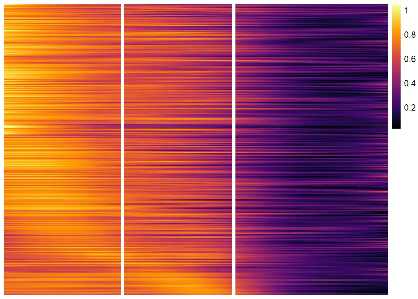
Trajectory trends via heatmaps
Displaying the expression trends of too many variables in a lineplot gets unclear quite rapidly. In order to deal with several variables use plotTrajectoryHeatmap(). While the trajectory’s directory is still displayed from left to right the dynamic of the gene-sets’ expression values is now displayed by the gradual change of a row’s color instead of a line’s slope in a lineplot. The advantage of using heatmaps to display dynamic expression changes along trajectories becomes obvious when the number of variables to display rises.
descending_gene_sets <- dplyr::pull(descending_gene_sets, variables)

plotTrajectoryHeatmap(object = spata_obj,
                      trajectory_name = "tumor-layers",
                      variables = descending_gene_sets,
                      arrange_rows = "maxima",
                      show_row_names = FALSE, # gene set names are long...
                      split_columns = TRUE,
                      smooth_span = 0.5)
plotTrajectoryHeatmap(object = spata_obj,
                      trajectory_name = "tumor-layers",
                      variables = peaking_genes,
                      arrange_rows = "maxima",
                      show_row_names = FALSE, # gene set names are long...
                      split_columns = TRUE, # splits the heatmap
                      smooth_span = 0.5)
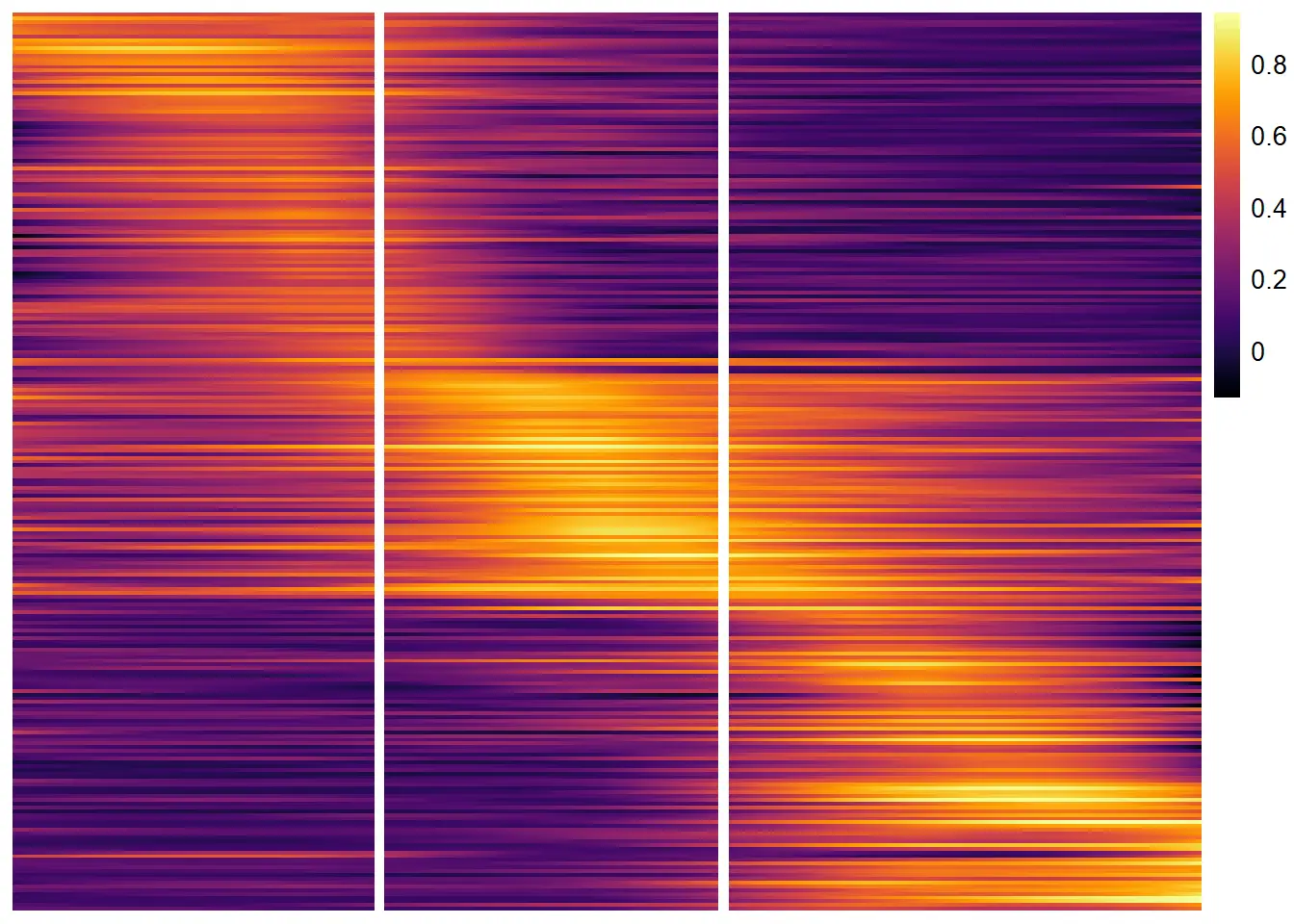
这个方法光看示例好像没什么优势,需要在实际中检验一下了,感觉整体效果不如stlearn

生活很好,有你更好


 889
889

 被折叠的 条评论
为什么被折叠?
被折叠的 条评论
为什么被折叠?
 到【灌水乐园】发言


