


- 🍨 本文为🔗365天深度学习训练营 中的学习记录博客
- 🍦 参考文章:Pytorch实战 | 第P4周:猴痘病识别
- 🍖 原作者:K同学啊 | 接辅导、项目定制
- 🚀 文章来源:K同学的学习圈子
一、前期准备
1.设置GPU
import torch
import torch.nn as nn
import matplotlib.pyplot as plt
from torchvision import transforms, datasets, models

device = torch.device("cuda" if torch.cuda.is_available() else "cpu")
print(device)
执行结果:
cuda
2.导入数据
import os,PIL,random,pathlib

data_dir = './data/'
data_dir = pathlib.Path(data_dir)
data_paths = list(data_dir.glob('*'))

classNames = [str(path).split("\\")[1] for path in data_paths]
print(classNames)
执行结果:
['Monkeypox', 'Others']
3.图像预处理和加载数据集
total_datadir = './data/'
train_transforms = transforms.Compose([
    transforms.Resize([224, 224]),      # 将输入图片resize成统一尺寸224 x 224
    transforms.ToTensor(),            # 转换为tensor格式, 并归一化
    transforms.Normalize(             # 标准化处理-->转换为标准正态分布(高斯分布),使模型更容易收敛
        mean=[0.485, 0.456, 0.406], # 用于图像标准化,RGB通道均值和标准差
        std=[0.229, 0.224, 0.225])
])

# 从total_datadir指定的目录加载图像数据,并使用train_transforms定义的转换来处理这些图像。加载后的数据集total_data会包含处理后的图像及其对应的标签。
total_data = datasets.ImageFolder(total_datadir, transform=train_transforms)
print(total_data)
print(total_data.class_to_idx) # 打印出一个字典,显示整数标签与实际类名之间的映射关系
执行结果:
Dataset ImageFolder             # 图像分类任务数据加载器
    Number of datapoints: 2142  # 数据集包含2142张图片
    Root location: ./data/
    StandardTransform  # 表示已对数据集应用了标准的转换
Transform: Compose(    # 应用于数据集的转换序列
               Resize(size=[224, 224], interpolation=bilinear, max_size=None, antialias=warn)   # 使用双线性插值方法进行缩放
               ToTensor()
               Normalize(mean=[0.485, 0.456, 0.406], std=[0.229, 0.224, 0.225])
           )

{'Monkeypox': 0, 'Others': 1}
4.划分数据集
train_size = int(0.8 * len(total_data))
test_size = len(total_data) - train_size

# torch.utils.data.random_split: 这是PyTorch提供的一个函数,用于将一个数据集随机分割为多个非重叠的新数据集。
train_dataset, test_dataset = torch.utils.data.random_split(total_data,[train_size, test_size])

print(train_dataset, test_dataset)
print(train_size, test_size)
执行结果:
成功从原始数据集中创建了两个子集,会显示这两个子集的内存地址。
<torch.utils.data.dataset.Subset object at 0x0000029E2CE57D60>
<torch.utils.data.dataset.Subset object at 0x0000029E2CE65970>

1713 429
5.数据加载器
在windows系统中需要将进程数设置为单进程,所以需要将数据处理部分DataLoader中的参数 num_workers设置为0或者采用默认为0的设置。
缺点:速度慢。
batch_size = 32
train_dl = torch.utils.data.DataLoader(train_dataset,
                                       batch_size=batch_size,
                                       shuffle=True)
test_dl = torch.utils.data.DataLoader(test_dataset,
                                      batch_size=batch_size,
                                      shuffle=True)
for imgs, labels in test_dl:  # imgs:数据加载器中输入数据(图像), # labels:数据的标签
	# N:批次中图像数量
	# C:图像通道数(RGB)
	# H:图像高度
	# W:图像宽度
    print("Shape of imgs [N, C, H, W]: ", imgs.shape)
    print("Shape of labels: ", labels.shape, labes.dtype) # 标签形状、标签数据类型
    break   # 只打印第一批
执行结果:
Shape of X [N, C, H, W]:  torch.Size([32, 3, 224, 224])
Shape of y:  torch.Size([32]) torch.int64
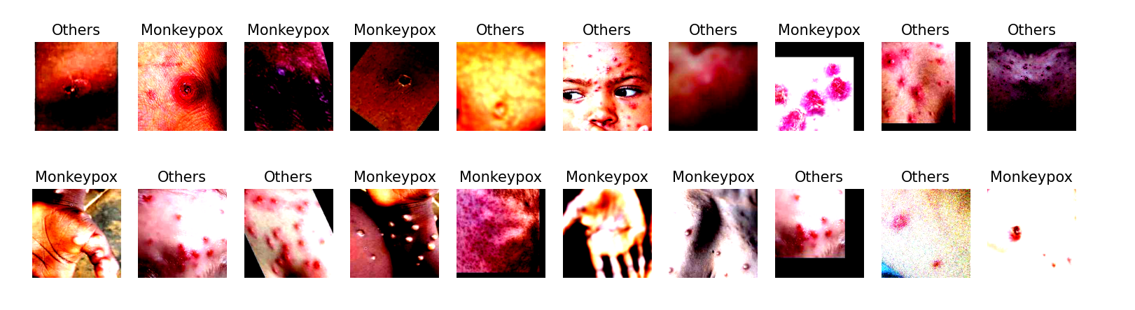
6.数据可视化【预警!!!!!!!!!!!!!!!!!】
plt.figure(figsize=(20,4))
for i in range(20):
    imgs, labels = train_dataset[i]
    plt.subplot(2, 10, i+1)
    plt.imshow(imgs.permute(1,2,0))
    plt.title(classNames[labels])
    plt.axis('off')

plt.show()
执行结果:
二、构建简单的CNN网络
import torch.nn.functional as F

class Network_bn(nn.Module):
    def __init__(self):
        super(Network_bn, self).__init__()
        self.conv1 = nn.Conv2d(in_channels=3, out_channels=12, kernel_size=5, stride=1, padding=0)
        self.bn1 = nn.BatchNorm2d(12)
        self.conv2 = nn.Conv2d(in_channels=12, out_channels=12, kernel_size=5, stride=1, padding=0)
        self.bn2 = nn.BatchNorm2d(12)
        self.pool = nn.MaxPool2d(2,2)
        self.conv4 = nn.Conv2d(in_channels=12, out_channels=24, kernel_size=5, stride=1, padding=0)
        self.bn4 = nn.BatchNorm2d(24)
        self.conv5 = nn.Conv2d(in_channels=24, out_channels=24, kernel_size=5, stride=1, padding=0)
        self.bn5 = nn.BatchNorm2d(24)
        self.fc1 = nn.Linear(24*50*50, len(classNames))

    def forward(self, x):
        x = F.relu(self.bn1(self.conv1(x)))
        x = F.relu(self.bn2(self.conv2(x)))
        x = self.pool(x)
        x = F.relu(self.bn4(self.conv4(x)))
        x = F.relu(self.bn5(self.conv5(x)))
        x = self.pool(x)
        x = x.view(-1, 24*50*50)
        x = self.fc1(x)

        return x

device = "cuda" if torch.cuda.is_available() else "cpu"
print("Using {} device".format(device))

model = Network_bn().to(device)
print(model)
执行结果:
Using cuda device
Network_bn(
  (conv1): Conv2d(3, 12, kernel_size=(5, 5), stride=(1, 1))
  (bn1): BatchNorm2d(12, eps=1e-05, momentum=0.1, affine=True, track_running_stats=True)
  (conv2): Conv2d(12, 12, kernel_size=(5, 5), stride=(1, 1))
  (bn2): BatchNorm2d(12, eps=1e-05, momentum=0.1, affine=True, track_running_stats=True)
  (pool): MaxPool2d(kernel_size=2, stride=2, padding=0, dilation=1, ceil_mode=False)
  (conv4): Conv2d(12, 24, kernel_size=(5, 5), stride=(1, 1))
  (bn4): BatchNorm2d(24, eps=1e-05, momentum=0.1, affine=True, track_running_stats=True)
  (conv5): Conv2d(24, 24, kernel_size=(5, 5), stride=(1, 1))
  (bn5): BatchNorm2d(24, eps=1e-05, momentum=0.1, affine=True, track_running_stats=True)
  (fc1): Linear(in_features=60000, out_features=2, bias=True)
)
三、训练模型
1.设置超参数
loss_fn = nn.CrossEntropyLoss() # 创建损失函数
learn_rate = 1e-4  # 学习率
opt = torch.optim.SGD(model.parameters(), lr=learn_rate)
2.编写训练函数
def train(dataloader, model, loss_fn, optimizer):
    size = len(dataloader.dataset) # 训练集大小
    num_batches = len(dataloader)  # 批次数目

    train_loss, train_acc = 0, 0   # 初始化训练损失和正确率

    for X, y in dataloader:  # 获取图片标签
        X, y = X.to(device), y.to(device)

        # 计算预测误差
        pred = model(X)
        loss = loss_fn(pred, y)

        # 反向传播
        optimizer.zero_grad()     # grad属性归零
        loss.backward()           # 反向传播
        optimizer.step()          # 每一步自动更新

        # 记录acc与loss
        train_acc += (pred.argmax(1) == y).type(torch.float).sum().item()
        train_loss += loss.item()

    train_acc /= size
    train_loss /= num_batches

    return train_acc, train_loss
3.编写测试函数
def test(dataloader, model, loss_fn):
    size = len(dataloader.dataset)         # 测试集大小
    num_batches = len(dataloader)  # 批次数目
    test_loss, test_acc = 0, 0

    # 当不进行训练是,停止梯度更新, 节省计算内存消耗
    with torch.no_grad():
        for imgs, target in dataloader:
            imgs, target = imgs.to(device), target.to(device)

            # 计算loss
            target_pred = model(imgs)
            loss = loss_fn(target_pred, target)

            test_loss += loss.item()
            test_acc += (target_pred.argmax(1) == target).type(torch.float).sum().item()

    test_acc /= size
    test_loss /= num_batches

    return test_acc, test_loss
4.正式训练
epochs = 20
train_loss = []
train_acc = []
test_loss = []
test_acc = []

for epoch in range(epochs):
    model.train()
    epoch_train_acc, epoch_train_loss = train(train_dl, model, loss_fn, opt)

    model.eval()
    epoch_test_acc, epoch_test_loss = test(test_dl, model, loss_fn)

    train_acc.append(epoch_train_acc)
    train_loss.append(epoch_train_loss)
    test_acc.append(epoch_test_acc)
    test_loss.append(epoch_test_loss)

    template = ('Epoch:{:2d}, Train_acc:{:.1f}%, Train_loss:{:.3f}, Test_acc:{:.1f}%, Test_loss:{:.3f}')
    print(template.format(epoch+1, epoch_train_acc*100, epoch_train_loss, epoch_test_acc*100, epoch_test_loss))
print('Done')
执行结果:
Epoch: 1, Train_acc:61.4%, Train_loss:0.673, Test_acc:68.5%, Test_loss:0.623
Epoch: 2, Train_acc:68.6%, Train_loss:0.597, Test_acc:69.2%, Test_loss:0.592
Epoch: 3, Train_acc:72.6%, Train_loss:0.547, Test_acc:72.3%, Test_loss:0.561
Epoch: 4, Train_acc:76.9%, Train_loss:0.506, Test_acc:73.9%, Test_loss:0.556
Epoch: 5, Train_acc:78.9%, Train_loss:0.478, Test_acc:78.1%, Test_loss:0.514
Epoch: 6, Train_acc:81.0%, Train_loss:0.445, Test_acc:69.5%, Test_loss:0.617
Epoch: 7, Train_acc:80.9%, Train_loss:0.432, Test_acc:78.3%, Test_loss:0.504
Epoch: 8, Train_acc:83.2%, Train_loss:0.407, Test_acc:77.9%, Test_loss:0.507
Epoch: 9, Train_acc:86.0%, Train_loss:0.378, Test_acc:78.6%, Test_loss:0.442
Epoch:10, Train_acc:86.5%, Train_loss:0.367, Test_acc:79.5%, Test_loss:0.439
Epoch:11, Train_acc:86.9%, Train_loss:0.356, Test_acc:80.0%, Test_loss:0.439
Epoch:12, Train_acc:88.1%, Train_loss:0.344, Test_acc:82.8%, Test_loss:0.429
Epoch:13, Train_acc:88.3%, Train_loss:0.329, Test_acc:80.7%, Test_loss:0.405
Epoch:14, Train_acc:89.4%, Train_loss:0.319, Test_acc:83.9%, Test_loss:0.402
Epoch:15, Train_acc:89.7%, Train_loss:0.306, Test_acc:84.6%, Test_loss:0.395
Epoch:16, Train_acc:90.7%, Train_loss:0.297, Test_acc:83.7%, Test_loss:0.386
Epoch:17, Train_acc:91.2%, Train_loss:0.285, Test_acc:84.6%, Test_loss:0.386
Epoch:18, Train_acc:91.6%, Train_loss:0.280, Test_acc:84.4%, Test_loss:0.374
Epoch:19, Train_acc:92.2%, Train_loss:0.274, Test_acc:83.7%, Test_loss:0.369
Epoch:20, Train_acc:92.3%, Train_loss:0.268, Test_acc:83.2%, Test_loss:0.449
Done
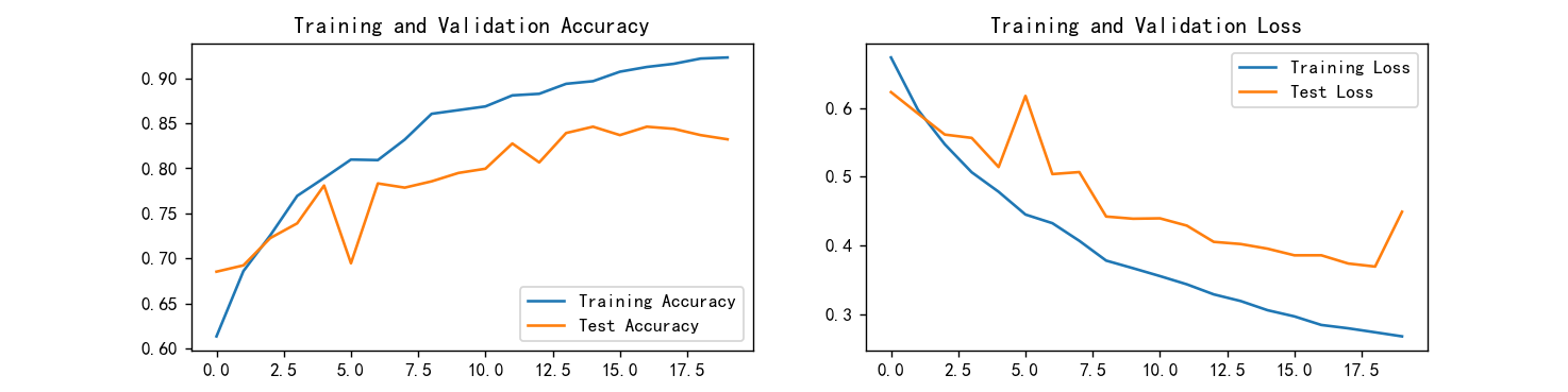
四、结果可视化
1.Loss与Accuracy图
import matplotlib.pyplot as plt
# 隐藏警告
import warnings
warnings.filterwarnings("ignore")             # 忽略警告信息
plt.rcParams['font.sans-serif'] = ['SimHei']  # 用来正常显示中文标签
plt.rcParams['axes.unicode_minus'] = False    # 用来正常显示负号
plt.rcParams['figure.dpi'] = 100              # 分辨率

epochs_range = range(epochs)

plt.figure(figsize=(12, 3))
plt.subplot(1, 2, 1)
plt.plot(epochs_range, train_acc, label='Training Accuracy')
plt.plot(epochs_range, test_acc, label='Test Accuracy')
plt.legend(loc='lower right')
plt.title('Training and Validation Accuracy')

plt.subplot(1, 2, 2)
plt.plot(epochs_range, train_loss, label='Training Loss')
plt.plot(epochs_range, test_loss, label='Test Loss')
plt.legend(loc='upper right')
plt.title('Training and Validation Loss')
plt.show()
执行结果:
2.指定图片进行预测
rom PIL import Image

classes = list(total_data.class_to_idx)

def predict_one_image(image_path, model, transform, classes):

    test_img = Image.open(image_path).convert('RGB')
    plt.imshow(test_img) # 展示预测图片

    test_img = transform(test_img)
    img = test_img.to(device).unsqueeze(0)

    model.eval()
    output = model(img)

    _,pred = torch.max(output, 1)
    pred_class = classes[pred]
    print(f'预测结果是:{pred_class}')
# 预测训练集中的某张图片(Monkeypox)
predict_one_image(image_path='data/Monkeypox/M01_01_00.jpg',
                  model=model,
                  transform=train_transforms,
                  classes=classes)

# 预测训练集中的某张图片(Others)
predict_one_image(image_path='data/Others/NM01_01_00.jpg',
                  model=model,
                  transform=train_transforms,
                  classes=classes)
执行结果:
预测结果是:Monkeypox
预测结果是:Others
五、保存并加载模型
PATH = './model.pth'   # 保存的参数文件名
torch.save(model.state_dict(), PATH)

# 将参数加载到model当中
model.load_state_dict(torch.load(PATH, map_location=device))
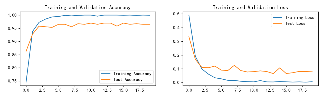
六、模型优化
尝试采用ResNet(Redidual Networks) :
class ResNetNetwork(nn.Module):
    def __init__(self):
        super(ResNetNetwork, self).__init__()
        self.resnet = models.resnet18(pretrained=True)
        num_ftrs = self.resnet.fc.in_features
        self.resnet.fc = nn.Linear(num_ftrs, len(classNames))

    def forward(self, x):
        x = self.resnet(x)
        return x

model = ResNetNetwork().to(device)
print(model)
修改学习率:
learn_rate = 1e-2 # 学习率
执行结果:
Epoch: 1, Train_acc:74.5%, Train_loss:0.491, Test_acc:86.2%, Test_loss:0.334
Epoch: 2, Train_acc:93.8%, Train_loss:0.191, Test_acc:92.8%, Test_loss:0.168
Epoch: 3, Train_acc:97.3%, Train_loss:0.099, Test_acc:95.8%, Test_loss:0.110
Epoch: 4, Train_acc:98.5%, Train_loss:0.062, Test_acc:95.6%, Test_loss:0.107
Epoch: 5, Train_acc:99.3%, Train_loss:0.035, Test_acc:95.3%, Test_loss:0.120
Epoch: 6, Train_acc:99.5%, Train_loss:0.027, Test_acc:96.5%, Test_loss:0.090
Epoch: 7, Train_acc:99.9%, Train_loss:0.016, Test_acc:96.5%, Test_loss:0.087
Epoch: 8, Train_acc:99.7%, Train_loss:0.016, Test_acc:95.6%, Test_loss:0.125
Epoch: 9, Train_acc:99.9%, Train_loss:0.009, Test_acc:96.7%, Test_loss:0.087
Epoch:10, Train_acc:100.0%, Train_loss:0.006, Test_acc:96.5%, Test_loss:0.077
Epoch:11, Train_acc:100.0%, Train_loss:0.005, Test_acc:97.0%, Test_loss:0.079
Epoch:12, Train_acc:99.6%, Train_loss:0.014, Test_acc:96.5%, Test_loss:0.085
Epoch:13, Train_acc:100.0%, Train_loss:0.005, Test_acc:97.0%, Test_loss:0.080
Epoch:14, Train_acc:100.0%, Train_loss:0.004, Test_acc:97.0%, Test_loss:0.065
Epoch:15, Train_acc:100.0%, Train_loss:0.007, Test_acc:95.8%, Test_loss:0.107
Epoch:16, Train_acc:99.9%, Train_loss:0.005, Test_acc:97.0%, Test_loss:0.065
Epoch:17, Train_acc:100.0%, Train_loss:0.003, Test_acc:96.5%, Test_loss:0.071
Epoch:18, Train_acc:99.9%, Train_loss:0.005, Test_acc:96.7%, Test_loss:0.081
Epoch:19, Train_acc:100.0%, Train_loss:0.003, Test_acc:96.5%, Test_loss:0.080
Epoch:20, Train_acc:99.9%, Train_loss:0.006, Test_acc:96.5%, Test_loss:0.078
Done


 589
589


 被折叠的 条评论
为什么被折叠?
被折叠的 条评论
为什么被折叠?
 到【灌水乐园】发言


