TPA_LSTM项目代码解读-pyrtoch

参考文章

论文地址
项目代码
TPA注意力机制(TPA-LSTM)
深度学习attention机制中的Q,K,V分别是从哪来的？

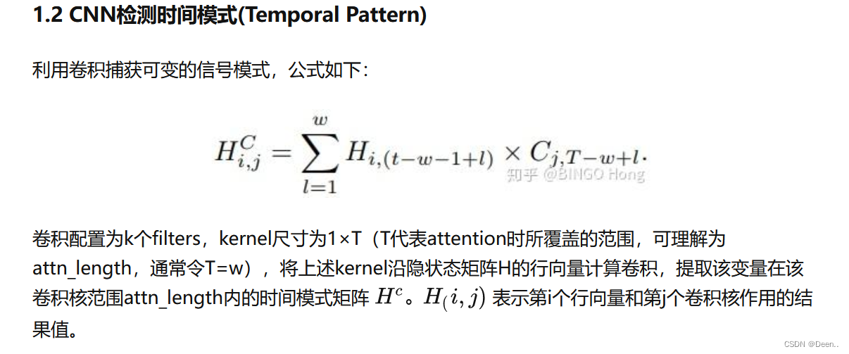
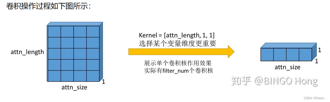
导读

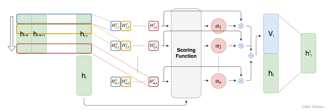
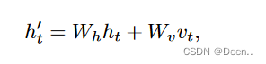
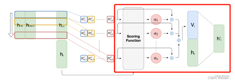
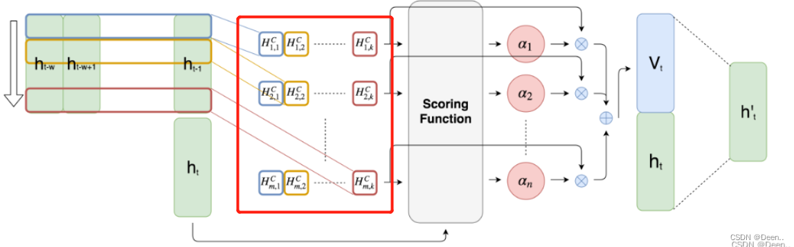
原文解释：图2提出的注意机制。ht表示RNN在时间步长t的隐藏状态。有k个长度为w的1-D CNN滤波器，用不同颜色的矩形表示。然后，每个滤波器对m个隐藏状态的特征进行卷积，并产生一个m行k列的矩阵HC。接下来，评分函数通过比较当前隐藏状态ht来计算每一行HC的权重。最后，对权重进行归一化，并对HC的行按其对应的权重进行加权求和，生成Vt。最后，我们将Vt、ht连接起来，并进行矩阵乘法，生成h, h用于创建最终的预测值。
TPA注意力机制(TPA-LSTM)简单的总结了这个模型的核心思想，作者用的tensorflow，本文介绍的项目代码是基于pytorch，可以直接在github上下载。
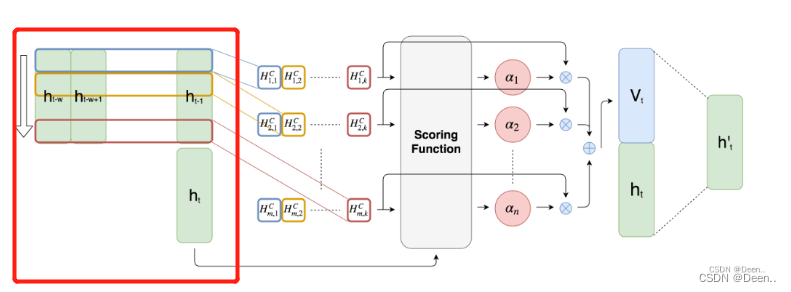
TPA-LSTM原理如图，简单来说就是，对原始时间序列使用LSTMBlockCell处理，得到上图中最左边绿色部分的$h_{t-w}$–$h_t$的隐藏状态。就是下图画红框的部分。

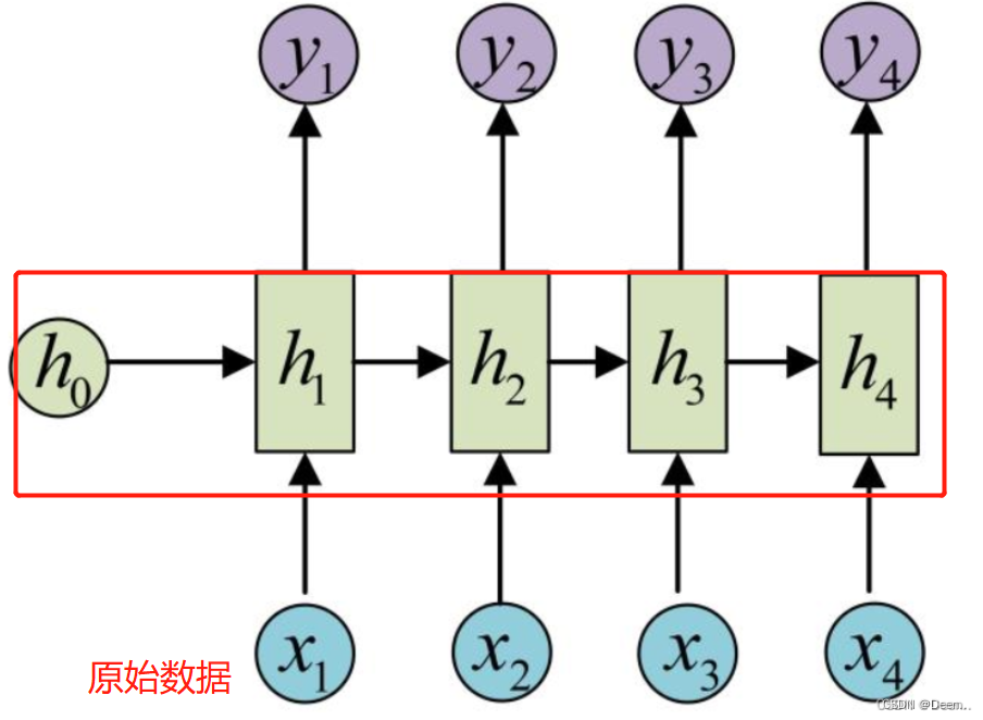
然后将这些隐藏态的$h$左右堆在一起，就变称了一个矩阵，下图红色部分。

再对这个矩阵进行CNN卷积，图中红色部分就是卷积的结果

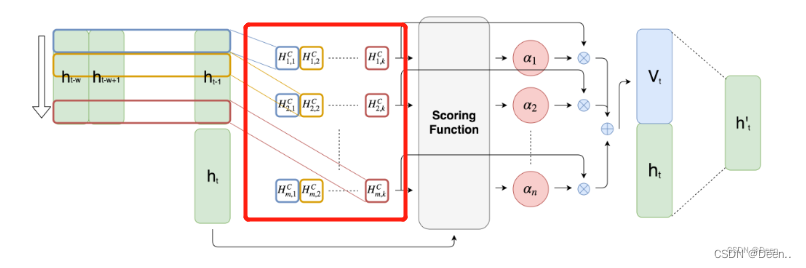
引用TPA注意力机制(TPA-LSTM)的总结：


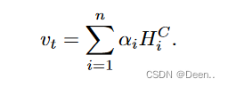
卷积后得到的数据就如上图画红框样子，然后进行注意力加权，用到的还是attention机制中的QKV，关于QKV的理解，可以参考深度学习attention机制中的Q,K,V分别是从哪来的？，将序列输出的最后一组$h_t$作为搜索序列$query$，将CNN卷积的结果作为$key$搜索用的关键信息，进行如下的公式计算后得到value，然后将v跟最开始的序列输出h_t加权后得到的结果就是模型最终输出结果。

参数配置

每个形参后都有英文介绍

parser = argparse.ArgumentParser(description='PyTorch Time series forecasting')
parser.add_argument('--data', type=str, default="data/exchange_rate.txt",
                    help='location of the data file')
#, required=True
parser.add_argument('--model', type=str, default='TPA_LSTM',
                    help='')
parser.add_argument('--hidden_state_features', type=int, default=12,
                    help='number of features in LSTMs hidden states')
parser.add_argument('--num_layers_lstm', type=int, default=1,
                    help='num of lstm layers')
parser.add_argument('--hidden_state_features_uni_lstm', type=int, default=1,
                    help='number of features in LSTMs hidden states for univariate time series')
parser.add_argument('--num_layers_uni_lstm', type=int, default=1,
                    help='num of lstm layers for univariate time series')
parser.add_argument('--attention_size_uni_lstm', type=int, default=10,
                    help='attention size for univariate lstm')
parser.add_argument('--hidCNN', type=int, default=10,
                    help='number of CNN hidden units')
parser.add_argument('--hidRNN', type=int, default=100,
                    help='number of RNN hidden units')
parser.add_argument('--window', type=int, default=24 * 7,
                    help='window size')
parser.add_argument('--CNN_kernel', type=int, default=1,
                    help='the kernel size of the CNN layers')
parser.add_argument('--highway_window', type=int, default=24,
                    help='The window size of the highway component')
parser.add_argument('--clip', type=float, default=10.,
                    help='gradient clipping')
parser.add_argument('--epochs', type=int, default=3000,
                    help='upper epoch limit') #30
parser.add_argument('--batch_size', type=int, default=128, metavar='N',
                    help='batch size')
parser.add_argument('--dropout', type=float, default=0.5,
                    help='dropout applied to layers (0 = no dropout)')
parser.add_argument('--seed', type=int, default=54321,
                    help='random seed')
parser.add_argument('--gpu', type=int, default=0)
parser.add_argument('--log_interval', type=int, default=2000, metavar='N',
                    help='report interval')
parser.add_argument('--save', type=str, default='model/model.pt',
                    help='path to save the final model')
parser.add_argument('--cuda', type=str, default=True)
parser.add_argument('--optim', type=str, default='adam')
parser.add_argument('--lr', type=float, default=1e-05)
parser.add_argument('--momentum', type=float, default=0.5)
parser.add_argument('--horizon', type=int, default=12)
parser.add_argument('--skip', type=float, default=24)
parser.add_argument('--hidSkip', type=int, default=5)
parser.add_argument('--L1Loss', type=bool, default=True)
parser.add_argument('--normalize', type=int, default=2)
parser.add_argument('--output_fun', type=str, default='sigmoid')
args = parser.parse_args()

读取数据

Data = Data_utility(args.data, 0.6, 0.2, args.cuda, args.horizon, args.window, args.normalize);

Data_utility类的行参：
def init(self, file_name, train, valid, cuda, horizon, window, normalize = 2):

• file_name 文件的路径
• train 训练集的占比
• valid 验证集占比
• cuda 是否使用GPU训练
• horizon 时间戳的理想界限
• window 滑动窗口
• normalize 使用标准化的模式供3种标准化模式，normalize = 2是按行方向的最大值归一化。

引用LSTNet时间序列预测的解释：

在这篇文章中，我们关注多变量时间预测的任务。正式的说，给定一系列观察到的时间序列信号Y = {y(1),y(2)，…，y(T)},其中，yt∈Rn, n为变量维数，我们的目标是以滚动预测的方式预测一系列未来信号。为了预测y(T+h)，我们需要提供{y(1),y(2)，…，y(T)}的数据，其中h是当前时间戳的理想界限(horizon我不知道该如何翻译，暂且认为是一个极限值)。同样的，为了预测下一个时间戳的值y(T+h+1)，需要提供{y(1),y(2)，…，y(T),y(T+1)}。因此我们把时间戳T的输入矩阵表示为X(T)={y1,y2，…，yT}，这个矩阵的维度是R(n*T)。

class Data_utility(object):
    # train and valid is the ratio of training set and validation set. test = 1 - train - valid
    def __init__(self, file_name, train, valid, cuda, horizon, window, normalize = 2):
        self.cuda = cuda;
        self.P = window;
        self.h = horizon
        #打开数据
        fin = open(file_name);
        #读取数据
        self.rawdat = np.loadtxt(fin,delimiter=',');
        self.dat = np.zeros(self.rawdat.shape);
        self.n, self.m = self.dat.shape;
        self.normalize = 2
        self.scale = np.ones(self.m);
        #数据标准化
        self._normalized(normalize);
        #训练集跟验证集分割
        self._split(int(train * self.n), int((train+valid) * self.n), self.n);
        #浮点型便于运算
        #时序数据每个维度上的所有数，例如100组时序数据，1个时序数据有10维，self.scale获得的是这10个维度上所有的数。
        self.scale = torch.from_numpy(self.scale).float();
        tmp = self.test[1] * self.scale.expand(self.test[1].size(0), self.m);

        if self.cuda:
            self.scale = self.scale.cuda();
        self.scale = Variable(self.scale);
        #标准化
        self.rse = normal_std(tmp);
        #相对绝对值误差
        self.rae = torch.mean(torch.abs(tmp - torch.mean(tmp)));

数据标准化

    def _normalized(self, normalize):
        #normalized by the maximum value of entire matrix.
       #不做标准化处理
        if (normalize == 0):
            self.dat = self.rawdat
        #找到数据集中的最大值，以它做标标准化
        if (normalize == 1):
            self.dat = self.rawdat / np.max(self.rawdat);
            
        #normlized by the maximum value of each row(sensor).
        #行方向最大值归一化
        if (normalize == 2):
            for i in range(self.m):
                #取出这一列的数值
                self.scale[i] = np.max(np.abs(self.rawdat[:,i]));
                #找到这一列的最大值，将这一列上的每个值都做相对这一列最大值的标准化
                self.dat[:,i] = self.rawdat[:,i] / np.max(np.abs(self.rawdat[:,i]));
            

数据集分类

给定一系列观察到的时间序列信号Y = {y(1),y(2)，…，y(T)},其中，yt∈Rn, n为变量维数，我们的目标是以滚动预测的方式预测一系列未来信号。为了预测y(T+h)，我们需要提供{y(1),y(2)，…，y(T)}的数据，其中h是当前时间戳的理想界限(horizon我不知道该如何翻译，暂且认为是一个极限值)。同样的，为了预测下一个时间戳的值y(T+h+1)，需要提供{y(1),y(2)，…，y(T),y(T+1)}。因此我们把时间戳T的输入矩阵表示为X(T)={y1,y2，…，yT}，这个矩阵的维度是R(n*T)。

图画的有点潦草，大致就是，多维序列（图中是2维）取一个window的数据作为输入数据，再取window长度+horizon处的数据，作为训练时求解损失函数的真实值，这样子训练出来的模型，也是那window中的数据，预测经过horizon数据戳后的数据值的情况。数据集按这种方式，向下滑动，window统一向下移动一格，对应的真实值部分也向下移动一格，如途中蓝色框所示。

        self._split(int(train * self.n), int((train+valid) * self.n), self.n);

    def _split(self, train, valid, test):
        
        train_set = range(self.P+self.h-1, train); #时间戳的极限+滑动窗口开始
        valid_set = range(train, valid);
        test_set = range(valid, self.n);
        self.train = self._batchify(train_set, self.h);
        self.valid = self._batchify(valid_set, self.h);
        self.test = self._batchify(test_set, self.h);
        
        
    def _batchify(self, idx_set, horizon):
        
        n = len(idx_set);
        X = torch.zeros((n,self.P,self.m));#先做个容器，大小为【window，时序数据的维度】
        Y = torch.zeros((n,self.m));#y是求损失函数时用到的ground truth 大小为【总时序数据集数量，时序数据的维度】
        #将数据按滑动窗口【这里滑动窗口取24*7=168个】的形式一组组的装起来，
        for i in range(n):
            end = idx_set[i] - self.h + 1;
            start = end - self.P;
            X[i,:,:] = torch.from_numpy(self.dat[start:end, :]);
            #Y这里取的是时间戳horizon里的数据
            Y[i,:] = torch.from_numpy(self.dat[idx_set[i], :]);

        return [X, Y];

下列代码是训练前的常规准备：

#eval()去引号，其实就是TPA_LSTM.Model(args, Data)
model = eval(args.model).Model(args, Data);
if(args.cuda):
    model.cuda()


#print(dict(model.named_parameters()))
if args.L1Loss:#损失函数求解方法
    criterion = nn.L1Loss(size_average=False);
else:
    criterion = nn.MSELoss(size_average=False);
evaluateL2 = nn.MSELoss(size_average=False);
evaluateL1 = nn.L1Loss(size_average=False)
if args.cuda:
    criterion = criterion.cuda()
    evaluateL1 = evaluateL1.cuda();
    evaluateL2 = evaluateL2.cuda();
#模型总参数计算
nParams = sum([p.nelement() for p in model.parameters()])
print('* number of parameters: %d' % nParams)

#print(list(model.parameters())[0].grad)
list(model.parameters())
#optim = Optim.Optim(model.parameters(), args.optim, args.lr, args.clip,)
#优化器策略
optim = torch.optim.SGD(model.parameters(), lr=args.lr, momentum=args.momentum)  #.01 1e-05
best_val = 10000000;

模型训练与验证

try:
    print('begin training');
    # 开始训练
    for epoch in range(1, args.epochs+1):
        epoch_start_time = time.time()#统计时间
        # 正式开始训练，并返回训练损失值。
        train_loss = train(Data, Data.train[0], Data.train[1], model, criterion, optim, args.batch_size)
        #print(train_loss)
        # 验证集的损失值，相对误差，错误率求解
        val_loss, val_rae, val_corr = evaluate(Data, Data.valid[0], Data.valid[1], model, evaluateL2, evaluateL1, args.batch_size);
        print('| end of epoch {:3d} | time: {:5.2f}s | train_loss {:5.4f} | valid rse {:5.4f} | valid rae {:5.4f} | valid corr  {:5.4f}'.format(
                epoch, (time.time() - epoch_start_time), train_loss, val_loss, val_rae, val_corr))
        # Save the model if the validation loss is the best we've seen so far.
        # 保存最佳的模型
        if val_loss < best_val:
            # with open(args.save, 'wb') as f:
            #     torch.save(model, f)
            best_val = val_loss
        # 每五轮进行一次测试，计算测试集的准确率等
        if epoch % 5 == 0:
            test_acc, test_rae, test_corr = evaluate(Data, Data.test[0], Data.test[1], model, evaluateL2, evaluateL1,
                                                     args.batch_size);
            print("test rse {:5.4f} | test rae {:5.4f} | test corr {:5.4f}".format(test_acc, test_rae, test_corr))
#通过键盘退出训练
except KeyboardInterrupt:
    print('-' * 89)
    print('Exiting from training early')

开始训练

模型通过上述代码中的
train_loss = train(Data, Data.train[0], Data.train[1], model, criterion, optim, args.batch_size)进行训练，解读train函数：

def train(data, X, Y, model, criterion, optim, batch_size):
    model.train();#训练模式，会进行梯度下降
    total_loss = 0;#本轮训练的总损失
    n_samples = 0;#样本总数
    for X, Y in data.get_batches(X, Y, batch_size, True):#通过迭代器data.get_batches（）往外给处每批训练数据
        model.zero_grad();
        output = model(X);#模型输出对应批次的预测结果
        scale = data.scale.expand(output.size(0), data.m)
        loss = criterion(output * scale, Y * scale);#损失求解 默认用的L1loss 可修改
        loss.backward();#反向传播
        grad_norm = optim.step();#根据参数的梯度和超参数（如学习率）来更新模型的参数，从而使得损失函数最小化
        total_loss += loss.data.item();#将损失存起来
        n_samples += (output.size(0) * data.m);
    return total_loss / n_samples

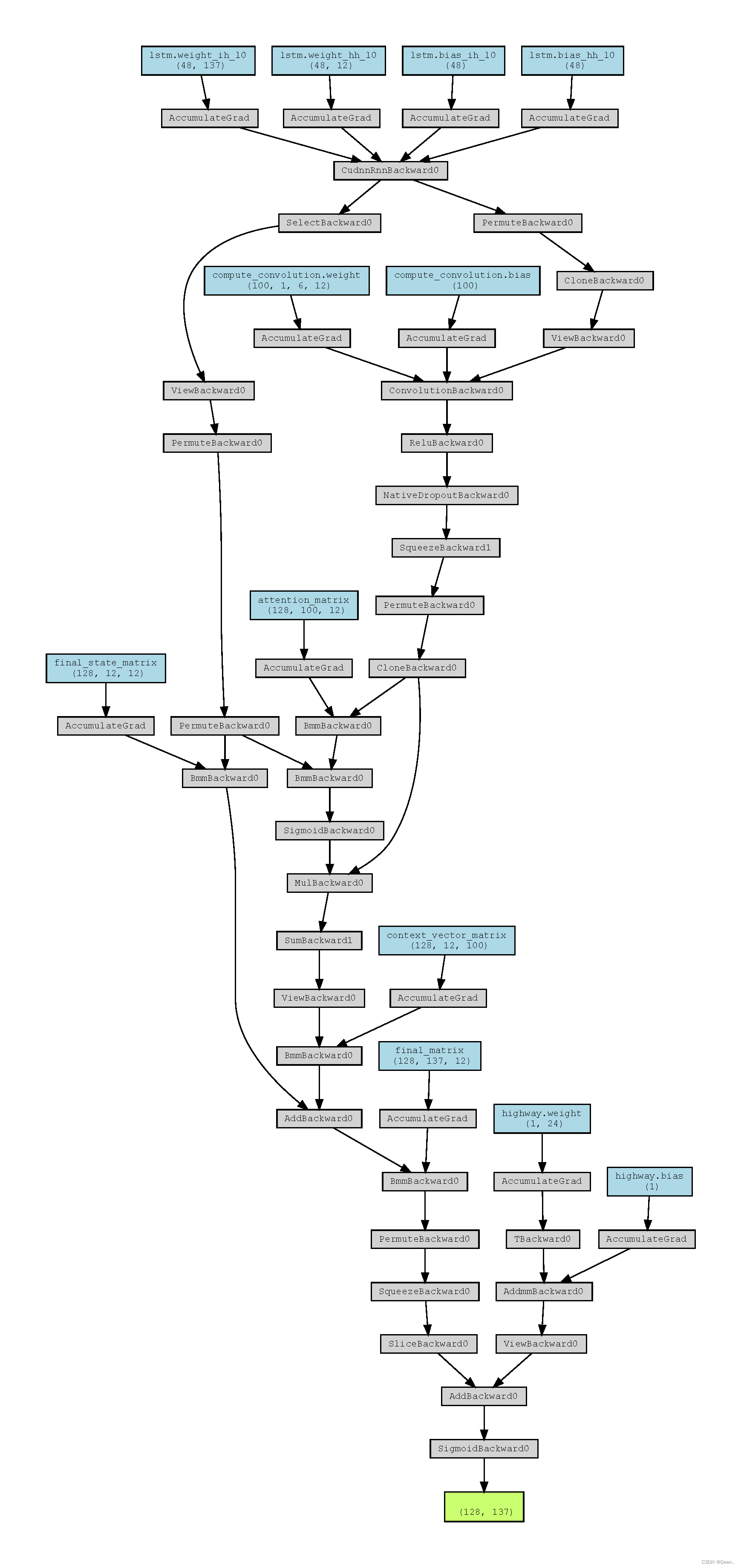
模型向前传播

下面是模型向前传播每一层情况：

===============================================================
out torch.Size([128, 137])
model Model(
  (lstm): LSTM(137, 12)
  (compute_convolution): Conv2d(1, 100, kernel_size=(6, 12), stride=(1, 1))
  (conv1): Conv2d(1, 100, kernel_size=(6, 137), stride=(1, 1))
  (GRU1): GRU(100, 100)
  (dropout): Dropout(p=0.2, inplace=False)
  (GRUskip): GRU(100, 5)
  (linear1): Linear(in_features=220, out_features=137, bias=True)
  (highway): Linear(in_features=24, out_features=1, bias=True)
)

• 首先将数据经LSTM处理

        #batch_first：True 或者 False，如果是 True，则 input 为(batch, seq, input_size)，默认值为：False（seq_len, batch, input_size）
        #bidirectional：如果设置为 True, 则表示双向 LSTM，默认为 False。
nn.LSTM(input_size=self.original_columns, hidden_size=self.hidden_state_features,
                            num_layers=self.num_layers_lstm,
                            bidirectional=False);

(lstm): LSTM(137, 12)

        ## input to lstm is of shape (seq_len, batch, input_size) (x shape (batch_size, seq_length, features))
        input_to_lstm = x.permute(1, 0, 2).contiguous()#LSTM的输入是(seq_len, batch, input_size),所以输入到LSTM中要转换一下维度
        #lstm_hidden_states记录下所有中间隐藏状态，h_all包含的是句子的最后一个单词的隐藏状态，c_all包含的是句子的最后一个单词的细胞状态，所以它们都与句子的长度seq_length无关。
        lstm_hidden_states, (h_all, c_all) = self.lstm(input_to_lstm)
        hn = h_all[-1].view(1, h_all.size(1), h_all.size(2))#最后一个隐藏态先存起来，后面做attention的时候用

对应下图操作

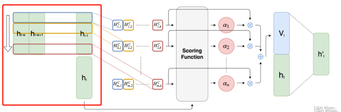
• 第二步CNN卷积处理 (compute_convolution): Conv2d(1, 100, kernel_size=(6, 12), stride=(1, 1))

            Step 2. Apply convolution on these hidden states. As in the paper TPA-LSTM, these filters are applied on the rows of the hidden state
        """
        output_realigned = lstm_hidden_states.permute(1, 0, 2).contiguous()
        hn = hn.permute(1, 0, 2).contiguous()
        # cn = cn.permute(1, 0, 2).contiguous()  #转为CNN卷积格式[batch,channal,w,h]
        input_to_convolution_layer = output_realigned.view(-1, 1, self.window_length, self.hidden_state_features);
        convolution_output = F.relu(self.compute_convolution(input_to_convolution_layer));
        convolution_output = self.dropout(convolution_output);#卷积激活再dropout

对应下两张图

• 第三步对卷积层使用注意力机制
  对卷积层做注意力时候，先判断最后一个隐藏态输出的尺寸是否原数据的数量一样多，如果不一样，就对卷积层跟最后一个隐藏态做填充：

        """
            Step 3. Apply attention on this convolution_output
        """
        convolution_output = convolution_output.squeeze(3)

        """
        在接下来的10行中，填充是为了使所有批大小相同，这样它们在矩阵乘法时就不会造成任何问题填充是必要的，以使所有批次的大小相等
        In the next 10 lines, padding is done to make all the batch sizes as the same so that they do not pose any problem while matrix multiplication
        padding is necessary to make all batches of equal size
        """
        final_hn = torch.zeros(self.attention_matrix.size(0), 1, self.hidden_state_features)
        final_convolution_output = torch.zeros(self.attention_matrix.size(0), self.hidC, self.window_length)
        diff = 0
        if (hn.size(0) < self.attention_matrix.size(0)):
            final_hn[:hn.size(0), :, :] = hn
            final_convolution_output[:convolution_output.size(0), :, :] = convolution_output
            diff = self.attention_matrix.size(0) - hn.size(0)
        else:
            final_hn = hn
            final_convolution_output = convolution_output

• 第四步，对隐藏态$h_t$跟隐藏态卷积结果做注意力计算
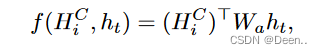
  这里的self.attention_matrix用的是torch,m.init,xavier uniform ，它是PyTorch中的-个初始化函数，用于初始化神经网络的权重参数。该函数根据论文"Understanding the dificulty of training deep feedforward neural networks"中的方法来初始化参数，该方法旨在使每层的输入和输出具有相同的方差。

           final_hn, final_convolution_output are the matrices to be used from here on
        """
        convolution_output_for_scoring = final_convolution_output.permute(0, 2, 1).contiguous()
        final_hn_realigned = final_hn.permute(0, 2, 1).contiguous()
        convolution_output_for_scoring = convolution_output_for_scoring.cuda()
        final_hn_realigned = final_hn_realigned.cuda()
        mat1 = torch.bmm(convolution_output_for_scoring, self.attention_matrix).cuda()
        scoring_function = torch.bmm(mat1, final_hn_realigned)
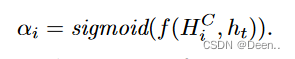
        alpha = torch.nn.functional.sigmoid(scoring_function)
        context_vector = alpha * convolution_output_for_scoring
        context_vector = torch.sum(context_vector, dim=1)

对应这两个公式跟图片




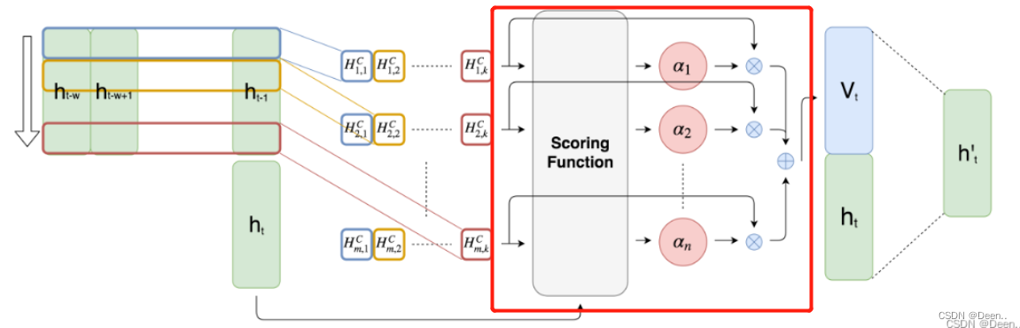
然后继续计算，按着文章的公式计算，其实文章的公式跟代码有一些不一样。

    """
           Step 4. Compute the output based upon final_hn_realigned, context_vector
        """
        context_vector = context_vector.view(-1, self.hidC, 1)
        h_intermediate = torch.bmm(self.final_state_matrix, final_hn_realigned) + torch.bmm(self.context_vector_matrix, context_vector)
        result = torch.bmm(self.final_matrix, h_intermediate)
        result = result.permute(0, 2, 1).contiguous()
        result = result.squeeze()

        """
           Remove from result the extra result points which were added as a result of padding 
        """
        final_result = result[:result.size(0) - diff]

• highway network
  这个项目里还加了highway network

        if (self.hw > 0):
            z = x[:, -self.hw:, :];
            z = z.permute(0, 2, 1).contiguous().view(-1, self.hw);
            z = self.highway(z);
            z = z.view(-1, self.original_columns);
            res = final_result + z;

        return torch.sigmoid(res)

预测阶段

预测阶段其实就是向数据输入模型，然后得到值，将值保存起来，这些得到的值就是预测值，相对训练阶段，少了一个梯度下降，反向传播过程。就略过。

        val_loss, val_rae, val_corr = evaluate(Data, Data.valid[0], Data.valid[1], model, evaluateL2, evaluateL1, args.batch_size);

def evaluate(data, X, Y, model, evaluateL2, evaluateL1, batch_size):
    model.eval();
    total_loss = 0;
    total_loss_l1 = 0;
    n_samples = 0;
    predict = None;
    test = None;

    for X, Y in data.get_batches(X, Y, batch_size, False):
        output = model(X);
        if predict is None:
            predict = output;
            test = Y;
        else:
            predict = torch.cat((predict, output));
            test = torch.cat((test, Y));

        scale = data.scale.expand(output.size(0), data.original_columns)
        total_loss += evaluateL2(output * scale, Y * scale).data
        total_loss_l1 += evaluateL1(output * scale, Y * scale).data
        n_samples += (output.size(0) * data.original_columns);
    rse = math.sqrt(total_loss / n_samples) / data.rse
    rae = (total_loss_l1 / n_samples) / data.rae

    predict = predict.data.cpu().numpy();
    Ytest = test.data.cpu().numpy();

    #print(predict.shape, Ytest.shape)

    sigma_p = (predict).std(axis=0);
    sigma_g = (Ytest).std(axis=0);
    mean_p = predict.mean(axis=0)
    mean_g = Ytest.mean(axis=0)
    index = (sigma_g != 0);
    correlation = ((predict - mean_p) * (Ytest - mean_g)).mean(axis=0) / (sigma_p * sigma_g);
    correlation = (correlation[index]).mean();
    return rse, rae, correlation;