Kaggle 便利店销量预测（xgboost附完整详细代码）

项目背景介绍

Forecast sales using store, promotion, and competitor data
Rossmann operates over 3,000 drug stores in 7 European countries. Currently,
Rossmann store managers are tasked with predicting their daily sales for up to six weeks in advance. Store sales are influenced by many factors, including promotions, competition, school and state holidays, seasonality, and locality. With thousands of individual managers predicting sales based on their unique circumstances, the accuracy of results can be quite varied.

In their first Kaggle competition, Rossmann is challenging you to predict 6 weeks of daily sales for 1,115 stores located across Germany. Reliable sales forecasts enable store managers to create effective staff schedules that increase productivity and motivation. By helping Rossmann create a robust prediction model, you will help store managers stay focused on what’s most important to them: their customers and their teams!If you are interested in joining Rossmann at their headquarters near Hanover, Germany, please contact Mr. Frank König (Frank.Koenig {at} rossmann.de) Rossmann is currently recruiting data scientists at senior and entry-level positions.

数据

You are provided with historical sales data for 1,115 Rossmann stores. The task is to forecast the “Sales” column for the test set. Note that some stores in the dataset were temporarily closed for refurbishment.

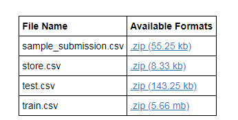
Files

train.csv - historical data including Sales
test.csv - historical data excluding Sales
sample_submission.csv - a sample submission file in the correct format
store.csv - supplemental information about the stores

Data fields

Most of the fields are self-explanatory. The following are descriptions for those that aren’t.

Id - an Id that represents a (Store, Date) duple within the test set
Store - a unique Id for each store
Sales - the turnover for any given day (this is what you are predicting)
Customers - the number of customers on a given day
Open - an indicator for whether the store was open: 0 = closed, 1 = open
StateHoliday - indicates a state holiday. Normally all stores, with few exceptions, are closed on state holidays. Note that all schools are closed on public holidays and weekends. a = public holiday, b = Easter holiday, c = Christmas, 0 = None
SchoolHoliday - indicates if the (Store, Date) was affected by the closure of public schools
StoreType - differentiates between 4 different store models: a, b, c, d
Assortment - describes an assortment level: a = basic, b = extra, c = extended
CompetitionDistance - distance in meters to the nearest competitor store
CompetitionOpenSince[Month/Year] - gives the approximate year and month of the time the nearest competitor was opened
Promo - indicates whether a store is running a promo on that day
Promo2 - Promo2 is a continuing and consecutive promotion for some stores: 0 = store is not participating, 1 = store is participating
Promo2Since[Year/Week] - describes the year and calendar week when the store started participating in Promo2
PromoInterval - describes the consecutive intervals Promo2 is started, naming the months the promotion is started anew. E.g. “Feb,May,Aug,Nov” means each round starts in February, May, August, November of any given year for that store

简单说明：

本项目根据给定的训练数据及各商店的一些基本信息，提取相关特征，从而构建训练数据集。给定的有1115家商店的历史销售数据，来预测未来6周的销量，以给商店销售作为参考。

导入数据

#导入需要的库
import numpy as np
import pandas as pd
import matplotlib.pyplot as plt
import seaborn as sns
%matplotlib inline
import xgboost as xgb
from time import time

#导入数据集
store=pd.read_csv(r'E:\python\data\store.csv')
train=pd.read_csv(r'E:\python\data\train.csv',dtype={'StateHoliday':pd.np.string_})
test=pd.read_csv(r'E:\python\data\test.csv',dtype={'StateHoliday':pd.np.string_})
#可以看前几行观察下数据的基本情况
store.head()
train.head()
test.head()

查看数据缺失情况：

#train数据无缺失
train.isnull().sum()

#test数据Open列有缺失
test.isnull().sum()
'''
Id                0
Store             0
DayOfWeek         0
Date              0
Open             11
Promo             0
StateHoliday      0
SchoolHoliday     0
dtype: int64
'''
#查看test缺失列都来自于622号店
test[test['Open'].isnull()]
#通过查看train里622号店的营业情况发现，622号店周一到周六都是营业的
train[train['Store']==622]
#所以我们认为缺失的部分是应该正常营业的，用1填充
test.fillna(1,inplace=True)

#store列缺失值较多，但数量看来比较一致，看一下是否同步缺失
store.isnull().sum()
'''
Store                          0
StoreType                      0
Assortment                     0
CompetitionDistance            3
CompetitionOpenSinceMonth    354
CompetitionOpenSinceYear     354
Promo2                         0
Promo2SinceWeek              544
Promo2SinceYear              544
PromoInterval                544
dtype: int64
'''
#下面是观察store缺失的情况
a1='CompetitionDistance'
a2='CompetitionOpenSinceMonth'
a3='CompetitionOpenSinceYear'
a4='Promo2SinceWeek'
a5='Promo2SinceYear'
a6='PromoInterval'
#a2和a3是同时缺失
store[(store[a2].isnull())&(store[a3].isnull())].shape
'''
(354, 10)
'''
#a4,a5,a6也是同时缺失
store[(store[a4].isnull())&(store[a5].isnull())&(store[a6].isnull())].shape
'''
(544, 10)
'''
#a4,a5,a6列缺失是因为没有活动
set(store[(store[a4].isnull())&(store[a5].isnull())&(store[a6].isnull())]['Promo2'])
'''
{0}
'''
#下面对缺失数据进行填充
#店铺竞争数据缺失，而且缺失的都是对应的。原因不明，而且数量也比较多，如果用中值或均值来填充，有失偏颇。暂且填0，解释意义就是刚开业
#店铺促销信息的缺失是因为没有参加促销活动，所以我们以0填充
store.fillna(0,inplace=True)

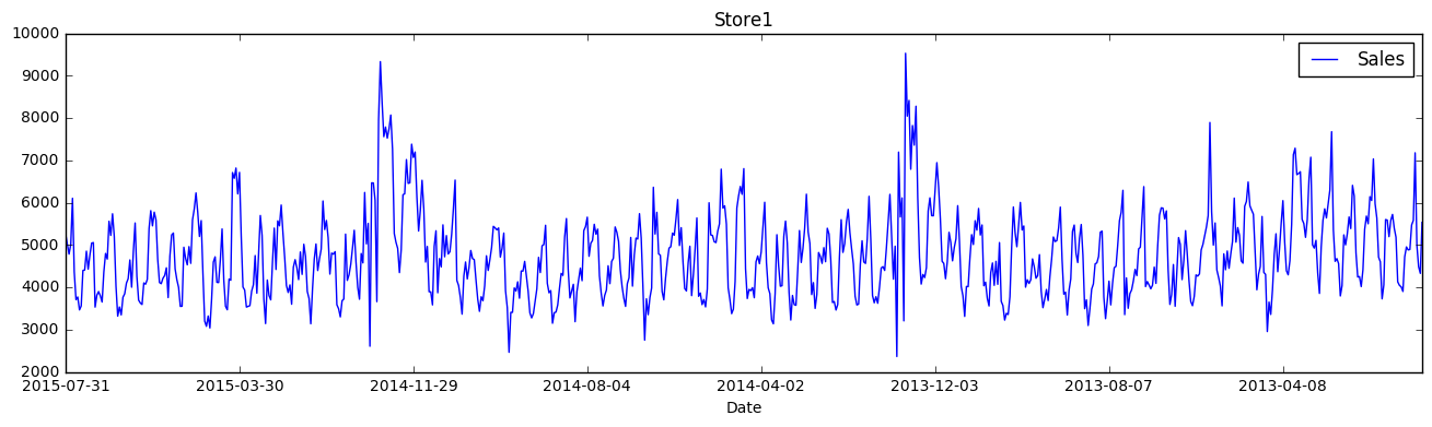
下面了解下销量随时间变化的情况：

#分析店铺销量随时间的变化
strain=train[train['Sales']>0]
strain.loc[strain['Store']==1,['Date','Sales']].plot(x='Date',y='Sales',title='Store1',figsize=(16,4))
#从图中可以看出店铺的销售额是有周期性变化的，一年中11,12月份销量相对较高，可能是季节因素或者促销等原因
#此外从2014年6-9月份的销量来看，6,7月份的销售趋势与8,9月份类似，而我们需要预测的6周在2015年8,9月份，因此我们可以把2015年6,7月份最近6周的1115家店的数据留出作为测试数据，用于模型的优化和验证

合并数据集：

上面需要的三个数据集缺失值也都处理完了，下面进行合并

#我们只需要销售额大于0的数据
train=train[train['Sales']>0]
#把store基本信息合并到训练和测试数据集上
train=pd.merge(train,store,on='Store',how='left')
test=pd.merge(test,store,on='Store',how='left')

train.info()
'''
<class 'pandas.core.frame.DataFrame'>
Int64Index: 844338 entries, 0 to 844337
Data columns (total 18 columns):
Store                        844338 non-null int64
DayOfWeek                    844338 non-null int64
Date                         844338 non-null object
Sales                        844338 non-null int64
Customers                    844338 non-null int64
Open                         844338 non-null int64
Promo                        844338 non-null int64
StateHoliday                 844338 non-null object
SchoolHoliday                844338 non-null int64
StoreType                    844338 non-null object
Assortment                   844338 non-null object
CompetitionDistance          844338 non-null float64
CompetitionOpenSinceMonth    844338 non-null float64
CompetitionOpenSinceYear     844338 non-null float64
Promo2                       844338 non-null int64
Promo2SinceWeek              844338 non-null float64
Promo2SinceYear              844338 non-null float64
PromoInterval                844338 non-null object
dtypes: float64(5), int64(8), object(5)
memory usage: 122.4+ MB
'''

特征工程

for data in [train,test]:
	#将时间特征进行拆分和转化
    data['year']=data['Date'].apply(lambda x:x.split('-')[0])
    data['year']=data['year'].astype(int)
    data['month']=data['Date'].apply(lambda x:x.split('-')[1])
    data['month']=data['month'].astype(int)
    data['day']=data['Date'].apply(lambda x:x.split('-')[2])
    data['day']=data['day'].astype(int)
	#将'PromoInterval'特征转化为'IsPromoMonth'特征，表示某天某店铺是否处于促销月，1表示是，0表示否
	#提示下：这里尽量不要用循环，用这种广播的形式，会快很多。循环可能会让你等的想哭
    month2str={1:'Jan',2:'Feb',3:'Mar',4:'Apr',5:'May',6:'Jun',7:'Jul',8:'Aug',9:'Sep',10:'Oct',11:'Nov',12:'Dec'}
    data['monthstr']=data['month'].map(month2str)
    data['IsPromoMonth']=data.apply(lambda x:0 if x['PromoInterval']==0 else 1 if x['monthstr'] in x['PromoInterval'] else 0,axis=1)
	#将存在其它字符表示分类的特征转化为数字
	mappings={'0':0,'a':1,'b':2,'c':3,'d':4}
    data['StoreType'].replace(mappings,inplace=True)
    data['Assortment'].replace(mappings,inplace=True)
    data['StateHoliday'].replace(mappings,inplace=True)

构建训练及测试数据集

#删掉训练和测试数据集中不需要的特征
df_train=train.drop(['Date','Customers','Open','PromoInterval','monthstr'],axis=1)
df_test=test.drop(['Id','Date','Open','PromoInterval','monthstr'],axis=1)
#如上所述，保留训练集中最近六周的数据用于后续模型的测试
Xtrain=df_train[6*7*1115:]
Xtest=df_train[:6*7*1115]

分析训练数据集中特征相关性

plt.subplots(figsize=(24,20))
sns.heatmap(df_train.corr(),cmap='RdYlGn',annot=True,vmin=-0.1,vmax=0.1,center=0)

提取后续用于模型训练的数据集：

#拆分特征与标签，并将标签取对数处理
ytrain=np.log1p(Xtrain['Sales'])
ytest=np.log1p(Xtest['Sales'])

Xtrain=Xtrain.drop(['Sales'],axis=1)
Xtest=Xtest.drop(['Sales'],axis=1)

模型构建

定义评价函数

#定义评价函数，可以传入后面模型中替代模型本身的损失函数
def rmspe(y,yhat):
    return np.sqrt(np.mean((yhat/y-1)**2))

def rmspe_xg(yhat,y):
    y=np.expm1(y.get_label())
    yhat=np.expm1(yhat)
    return 'rmspe',rmspe(y,yhat)

构建初始模型

#初始模型构建
#参数设定
params={'objective':'reg:linear',
       'booster':'gbtree',
       'eta':0.03,
       'max_depth':10,
       'subsample':0.9,
       'colsample_bytree':0.7,
       'silent':1,
       'seed':10}
num_boost_round=6000
dtrain=xgb.DMatrix(Xtrain,ytrain)
dvalid=xgb.DMatrix(Xtest,ytest)
watchlist=[(dtrain,'train'),(dvalid,'eval')]

#模型训练
print('Train a XGBoost model')
start=time()
gbm=xgb.train(params,dtrain,num_boost_round,evals=watchlist,
             early_stopping_rounds=100,feval=rmspe_xg,verbose_eval=True)
end=time()
print('Train time is {:.2f} s.'.format(end-start))
'''
Train time is 3019.86 s.
数据集有点大，训练就花了50分钟。。
'''

结果分析：

#采用保留数据集进行检测
print('validating')
Xtest.sort_index(inplace=True)
ytest.sort_index(inplace=True)
yhat=gbm.predict(xgb.DMatrix(Xtest))
error=rmspe(np.expm1(ytest),np.expm1(yhat))
print('RMSPE: {:.6f}'.format(error))
'''
validating
RMSPE: 0.128683
'''

#构建保留数据集预测结果
res=pd.DataFrame(data=ytest)
res['Predicition']=yhat
res=pd.merge(Xtest,res,left_index=True,right_index=True)
res['Ratio']=res['Predicition']/res['Sales']
res['Error']=abs(res['Ratio']-1)
res['Weight']=res['Sales']/res['Predicition']
res.head()

#分析保留数据集中任意三个店铺的预测结果
col_1=['Sales','Predicition']
col_2=['Ratio']
L=np.random.randint(low=1,high=1115,size=3)
print('Mean Ratio of predition and real sales data is {}:store all'.format(res['Ratio'].mean()))
for i in L:
    s1=pd.DataFrame(res[res['Store']==i],columns=col_1)
    s2=pd.DataFrame(res[res['Store']==i],columns=col_2)
    s1.plot(title='Comparation of predition and real sales data:store {}'.format(i),figsize=(12,4))
    s2.plot(title='Ratio of predition and real sales data: store {}'.format(i),figsize=(12,4))
    print('Mean Ratio of predition and real sales data is {}:store {}'.format(s2['Ratio'].mean(),i))
'''
Mean Ratio of predition and real sales data is 1.0020524030390718:store all
Mean Ratio of predition and real sales data is 1.006614925026921:store 181
Mean Ratio of predition and real sales data is 1.0024662925685335:store 1078
Mean Ratio of predition and real sales data is 1.0020672433947455:store 911
图片有些大，我就不粘上来了
'''

#分析偏差最大的10个预测结果
res.sort_values(['Error'],ascending=False,inplace=True)
res[:10]

#从分析结果来看，初始模型已经可以比较好的预测保留数据集的销售趋势，但相对真实值，模型的预测值整体要偏高一些。从对偏差数据分析来看，偏差最大的3个数据也是明显偏高。因此，我们可以以保留数据集为标准对模型进行偏差校正。

模型优化：

#偏差整体校正优化
print('weight correction')
W=[(0.990+(i/1000)) for i in range(20)]
S=[]
for w in W:
    error=rmspe(np.expm1(ytest),np.expm1(yhat*w))
    print('RMSPE for {:.3f}:{:.6f}'.format(w,error))
    S.append(error)
Score=pd.Series(S,index=W)
Score.plot()
BS=Score[Score.values==Score.values.min()]
print('Best weight for Score:{}'.format(BS))
'''
weight correction
RMSPE for 0.990:0.131899
RMSPE for 0.991:0.129076
RMSPE for 0.992:0.126723
……
Best weight for Score:0.996    0.122779
dtype: float64
'''
#当校正系数为0.996时，保留数据集的RMSPE得分最低：0.122779,相对于初始模型0.128683得分有很大的提升。
#因为每个店铺都有自己的特点，而我们设计的模型对不同的店铺偏差并不完全相同，所以我们需要根据不同的店铺进行一个细致的校正。

#细致校正：以不同的店铺分组进行细致校正，每个店铺分别计算可以取得最佳RMSPE得分的校正系数
L=range(1115)
W_ho=[]
W_test=[]
for i in L:
    s1=pd.DataFrame(res[res['Store']==i+1],columns=col_1)
    s2=pd.DataFrame(df_test[df_test['Store']==i+1])
    W1=[(0.990+(i/1000)) for i in range(20)]
    S=[]
    for w in W1:
        error=rmspe(np.expm1(s1['Sales']),np.expm1(s1['Predicition']*w))
        S.append(error)
    Score=pd.Series(S,index=W1)
    BS=Score[Score.values==Score.values.min()]
    a=np.array(BS.index.values)
    b_ho=a.repeat(len(s1))
    b_test=a.repeat(len(s2))
    W_ho.extend(b_ho.tolist())
    W_test.extend(b_test.tolist())
#调整校正系数的排序
Xtest=Xtest.sort_values(by='Store')
Xtest['W_ho']=W_ho
Xtest=Xtest.sort_index()
W_ho=list(Xtest['W_ho'].values)
Xtest.drop(['W_ho'],axis=1,inplace=True)

df_test=df_test.sort_values(by='Store')
df_test['W_test']=W_test
df_test=df_test.sort_index()
W_test=list(df_test['W_test'].values)
df_test.drop(['W_test'],axis=1,inplace=True)

#计算校正后整体数据的RMSPE得分
yhat_new=yhat*W_ho
error=rmspe(np.expm1(ytest),np.expm1(yhat_new))
print('RMSPE for weight corretion {:.6f}'.format(error))
'''
RMSPE for weight corretion 0.116168
相对于整体校正的0.122779的得分又有不小的提高
'''

对测试数据进行预测并导出结果

#用初始和校正后的模型对训练数据集进行预测
print('Make predictions on the test set')
dtest=xgb.DMatrix(df_test)
test_probs=gbm.predict(dtest)

#初始模型
result=pd.DataFrame({'Id':test['Id'],'Sales':np.expm1(test_probs)})
result.to_csv(r'E:\python\data\result\Rossmann_submission_1.csv',index=False)
#整体校正模型
result=pd.DataFrame({'Id':test['Id'],'Sales':np.expm1(test_probs*0.996)})
result.to_csv(r'E:\python\data\result\Rossmann_submission_2.csv',index=False)
#细致校正模型
result=pd.DataFrame({'Id':test['Id'],'Sales':np.expm1(test_probs*W_test)})
result.to_csv(r'E:\python\data\result\Rossmann_submission_3.csv',index=False)

上面构建的模型经过优化后，已经有着不错的表现。如果想继续提高预测的精度，可以在模型融合上试试。本文下面通过构建多个xgboost模型，来构造融合模型。

模型融合

#训练融合模型：训练了10个模型并对偏差分别对每个店铺进行优化
#这里跑10个模型确实挺困难的，用笔记本跑了一整天，也可以减少几个试试。
#下面的代码跟上面模型构建的代码基本都是重复的
print('Train an new ensemble XGBoost model')
start=time()
rounds=10
preds_ho=np.zeros((len(Xtest.index),rounds))
preds_test=np.zeros((len(df_test.index),rounds))
B=[]
for r in range(rounds):
    print('round {}:'.format(r+1))
    
    params={'objective':'reg:linear',
       'booster':'gbtree',
       'eta':0.03,
       'max_depth':10,
       'subsample':0.9,
       'colsample_bytree':0.7,
       'silent':1,
       'seed':r+1}
    num_boost_round=6000
    gbm=xgb.train(params,dtrain,num_boost_round,evals=watchlist,
             early_stopping_rounds=100,feval=rmspe_xg,verbose_eval=True)
    
    yhat=gbm.predict(xgb.DMatrix(Xtest))
    #下面对每个店铺进行偏差优化
    L=range(1115)
    W_ho=[]
    W_test=[]
    for i in L:
        s1=pd.DataFrame(res[res['Store']==i+1],columns=col_1)
        s2=pd.DataFrame(df_test[df_test['Store']==i+1])
        W1=[(0.990+(i/1000)) for i in range(20)]
        S=[]
        for w in W1:
            error=rmspe(np.expm1(s1['Sales']),np.expm1(s1['Predicition']*w))
            S.append(error)
        Score=pd.Series(S,index=W1)
        BS=Score[Score.values==Score.values.min()]
        a=np.array(BS.index.values)
        b_ho=a.repeat(len(s1))
        b_test=a.repeat(len(s2))
        W_ho.extend(b_ho.tolist())
        W_test.extend(b_test.tolist())
    #重新调整权重顺序    
    Xtest=Xtest.sort_values(by='Store')
    Xtest['W_ho']=W_ho
    Xtest=Xtest.sort_index()
    W_ho=list(Xtest['W_ho'].values)
    Xtest.drop(['W_ho'],axis=1,inplace=True)

    df_test=df_test.sort_values(by='Store')
    df_test['W_test']=W_test
    df_test=df_test.sort_index()
    W_test=list(df_test['W_test'].values)
    df_test.drop(['W_test'],axis=1,inplace=True)
    
    yhat_ho=yhat*W_ho
    yhat_test=gbm.predict(xgb.DMatrix(df_test))*W_test
    error=rmspe(np.expm1(ytest),np.expm1(yhat_ho))
    B.append(error)
    preds_ho[:,r]=yhat_ho
    preds_test[:,r]=yhat_test
    print('round {} end'.format(r+1))
    
end=time()
time_elapsed=end-start
print('Training is end')
print('Training time is {} h.'.format(time_elapsed/3600))

#分析不同模型的相关性
preds=pd.DataFrame(preds_ho)
sns.pairplot(preds)
#模型融合可以采用简单平均或者加权重的方法进行融合。从上面图中看，这10个模型相关性很高，差别不大。所以权重融合我们只考虑训练中单独模型在保留数据集中的得分情况分配权重。

模型融合在保留数据集上的表现：

#简单平均融合
print('Validating')
bagged_ho_preds1=preds_ho.mean(axis=1)
error1=rmspe(np.expm1(ytest),np.expm1(bagged_ho_preds1))
print('RMSPE for mean: {:.6f}'.format(error1))
'''
Validating
RMSPE for mean: 0.114743
'''
#加权融合
R=range(10)
Mw=[0.20,0.20,0.10,0.10,0.10,0.10,0.10,0.10,0.00,0.00]
A=pd.DataFrame()
A['round']=R
A['best_score']=B
A.sort_values(['best_score'],inplace=True)
A['weight']=Mw
A.sort_values(['round'],inplace=True)
weight=np.array(A['weight'])
preds_ho_w=weight*preds_ho
bagged_ho_preds2=preds_ho_w.sum(axis=1)
error2=rmspe(np.expm1(ytest),np.expm1(bagged_ho_preds2))
print('RMSPE for weight: {:.6f}'.format(error2))
'''
RMSPE for weight: 0.114174
权重模型较均值模型有比较好的得分
'''

融合模型对训练集进行预测：

#用均值融合和加权融合后的模型对训练数据集进行预测
#均值融合
print('Make predictions on the test set')
bagged_preds=preds_test.mean(axis=1)
result=pd.DataFrame({'Id':test['Id'],'Sales':np.expm1(bagged_preds)})
result.to_csv(r'E:\python\data\result\Rossmann_submission_4.csv',index=False)
#加权融合
bagged_preds=(preds_test*weight).sum(axis=1)
result=pd.DataFrame({'Id':test['Id'],'Sales':np.expm1(bagged_preds)})
result.to_csv(r'E:\python\data\result\Rossmann_submission_5.csv',index=False)

下面对模型特征重要性及最佳模型结果进行分析：

#模型特征重要性
xgb.plot_importance(gbm)

从模型特征重要性分析，比较重要的特征有：
1.周期性特征：‘day’,‘month’,'year’等，可见店铺的销售额与时间是息息相关的，尤其是周期较短的时间特征。
2.店铺差异：‘store’,‘storetype’，不同店铺的销售额存在特异性。
3.短期促销情况：‘promo‘，促销会带来销售额的提升。
4.竞争对手相关特征。
作用不太大的特征：假期特征及持续促销特征。
以上分析对于后续的经营活动也有着很好的指导作用。

采用新的融合模型对于保留数据集的提升情况：

#采用新的权值融合模型构建保留数据集预测结果
res1=pd.DataFrame(data=ytest)
res1['Predicition']=bagged_ho_preds2
res1=pd.merge(Xtest,res1,left_index=True,right_index=True)
res1['Ratio']=res1['Predicition']/res1['Sales']
res1['Error']=abs(res1['Ratio']-1)
res1.head()

#分析偏差最大的10个预测结果与初始模型差异
res1.sort_values(['Error'],ascending=False,inplace=True)
res['Store_new']=res1['Store']
res['Error_new']=res1['Error']
res['Ratio_new']=res1['Ratio']
col_3=['Store','Ratio','Error','Store_new','Ratio_new','Error_new']
com=pd.DataFrame(res,columns=col_3)
com[:10]
#从新旧模型预测结果最大的几个偏差对比的情况来看，最终的融合模型在这几个预测值上大多有所提升，证明模型的校正和融合确实有效。