


notice:The detailed code is not presented in this article
1. For the polynomial f(x) = x^4 – 2*x^3 , calculate the derivative and the 2nd derivative analytically (the first derivative so that you can compare with your numerical derivatives to determine the error, and the second derivative might be useful for understanding your results—see equations (1.4) and (1.6)).
a) Choose different step sizes h and plot a log-log graph of error vs step size to compare the numerical derivatives found using the forward, backward, and central difference formulas with the actual derivative. How accurate are the numerical derivatives at x = 0, 1, 1.5, and 2? At what step sizes do you obtain the minimum errors, and what are the minimum errors (see Sauer figure 5.1)? Do you expect that this would be a problem? What if you were using single-precision floating point? (You can easily try this in Matlab by using the single() function.)
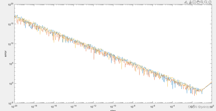
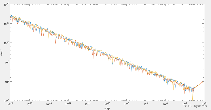
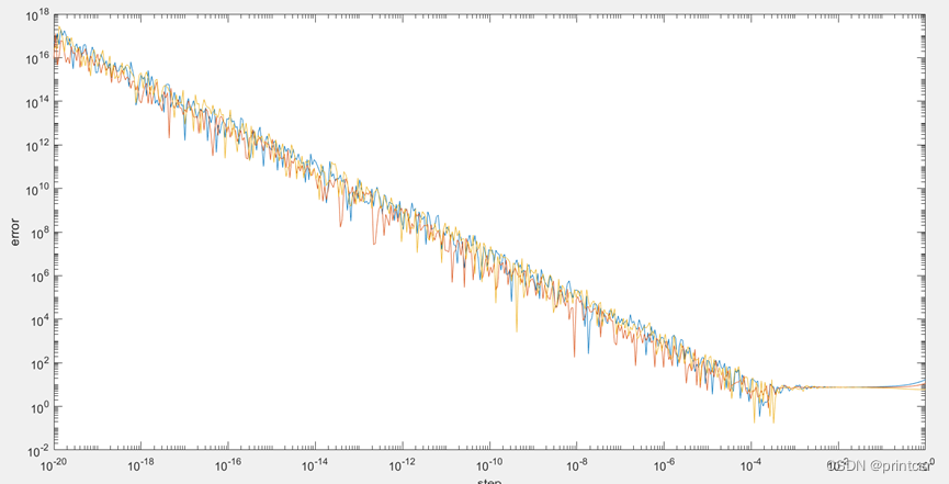
b) Add some additional error to your polynomial. For example, try y = f(x) + 0.001 * randn(size(x));. How does the error in the numerical derivative vary with step size h? Try changing the size of the error.
Checklist Did you differentiate the function (including with added error)? Did you explain how you did it? Did you plot graphs showing the error vs step size at each point? Are your graphs and axes properly labelled? Did you discuss whether the results were what you expected? Did you discuss any unusual results? Did you include code where appropriate? Did you reference the source of any code you didn’t write?
(1).result
1.the three function’s code(omitted)
2.find minimize h and different errors(omitted)
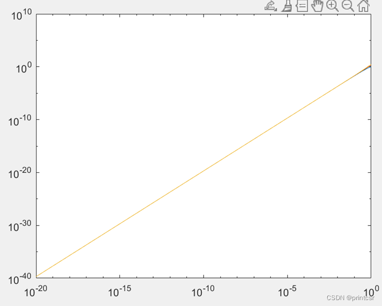
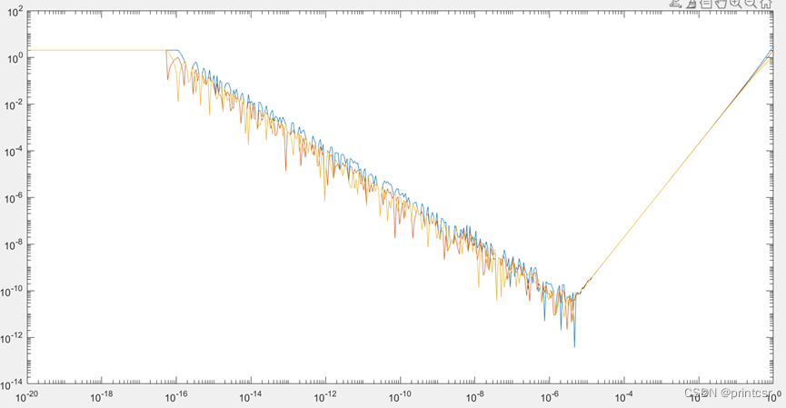
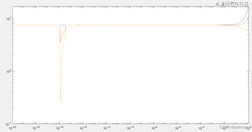
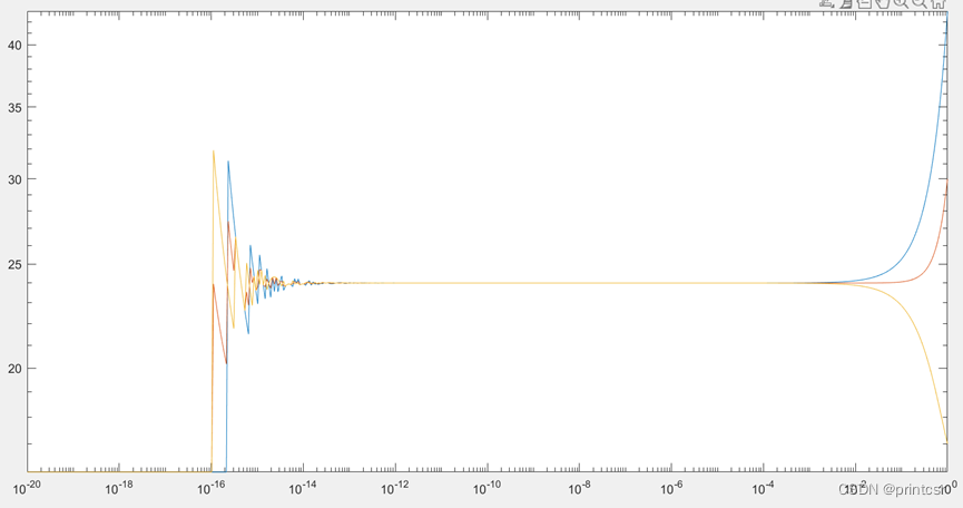
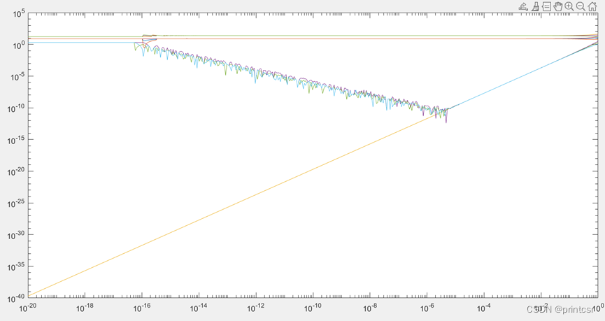
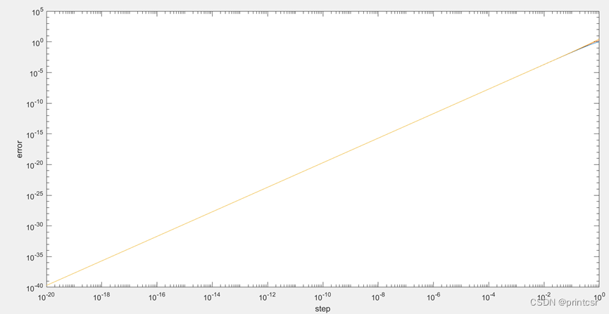
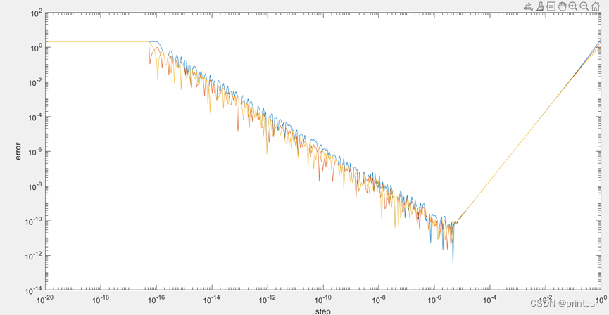
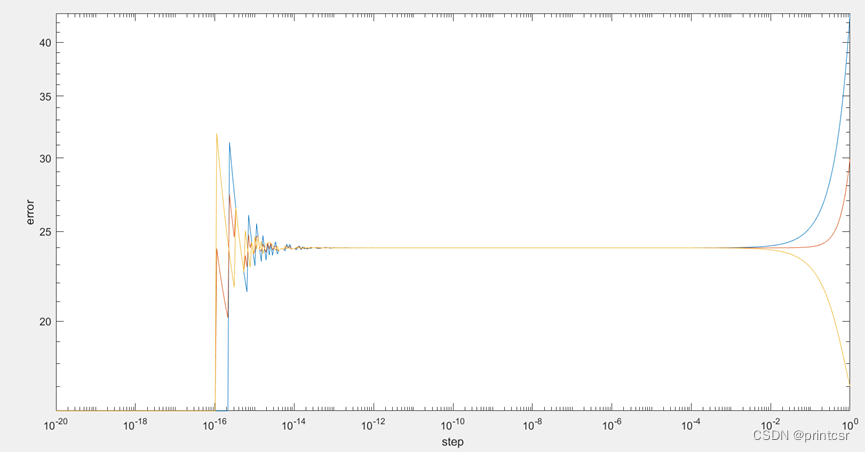
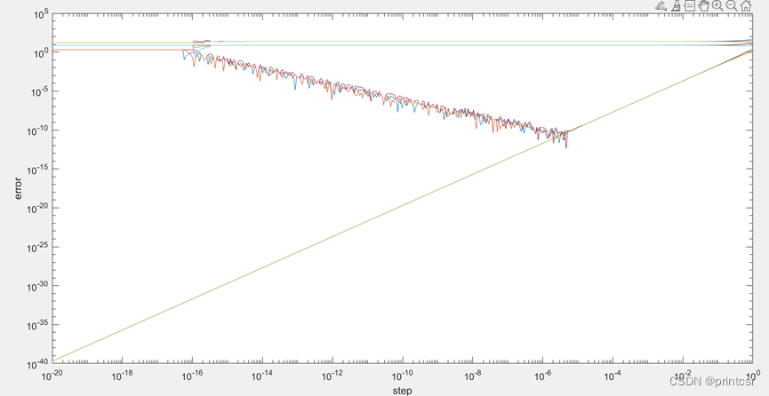
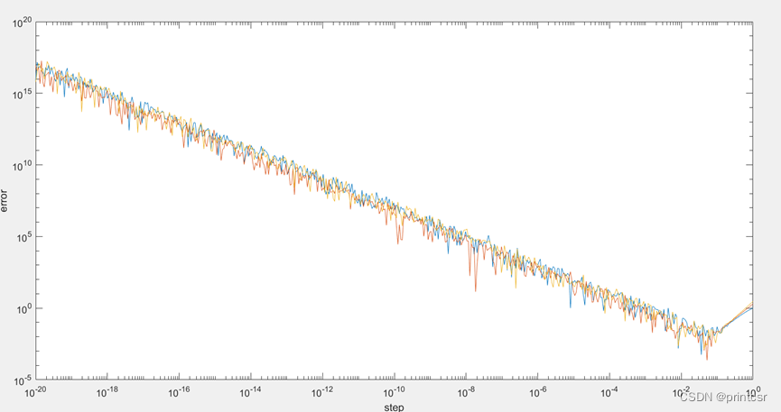
3..the log-log graph of error vs step size
the picture:
when x=0
When x=1
When x=1.5
when x=2
The total graph:
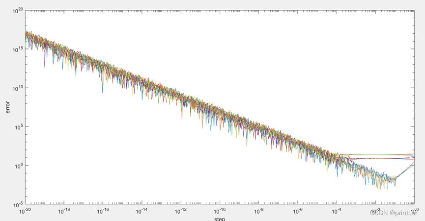
5. using single-precision floating point
picture:
when x=0
when x=1
 when x=1.5

when x=2
The total graph:
6.full project’s codes
(2).result
When x=0
when x=1
When x=1.5
 when x=2
The total graph:


 3920
3920


 被折叠的 条评论
为什么被折叠?
被折叠的 条评论
为什么被折叠?
 到【灌水乐园】发言


