


💥💥💞💞欢迎来到本博客❤️❤️💥💥
🏆博主优势:🌞🌞🌞博客内容尽量做到思维缜密,逻辑清晰,为了方便读者。
⛳️座右铭:行百里者,半于九十。
📋📋📋本文目录如下:🎁🎁🎁
目录

💥1 概述
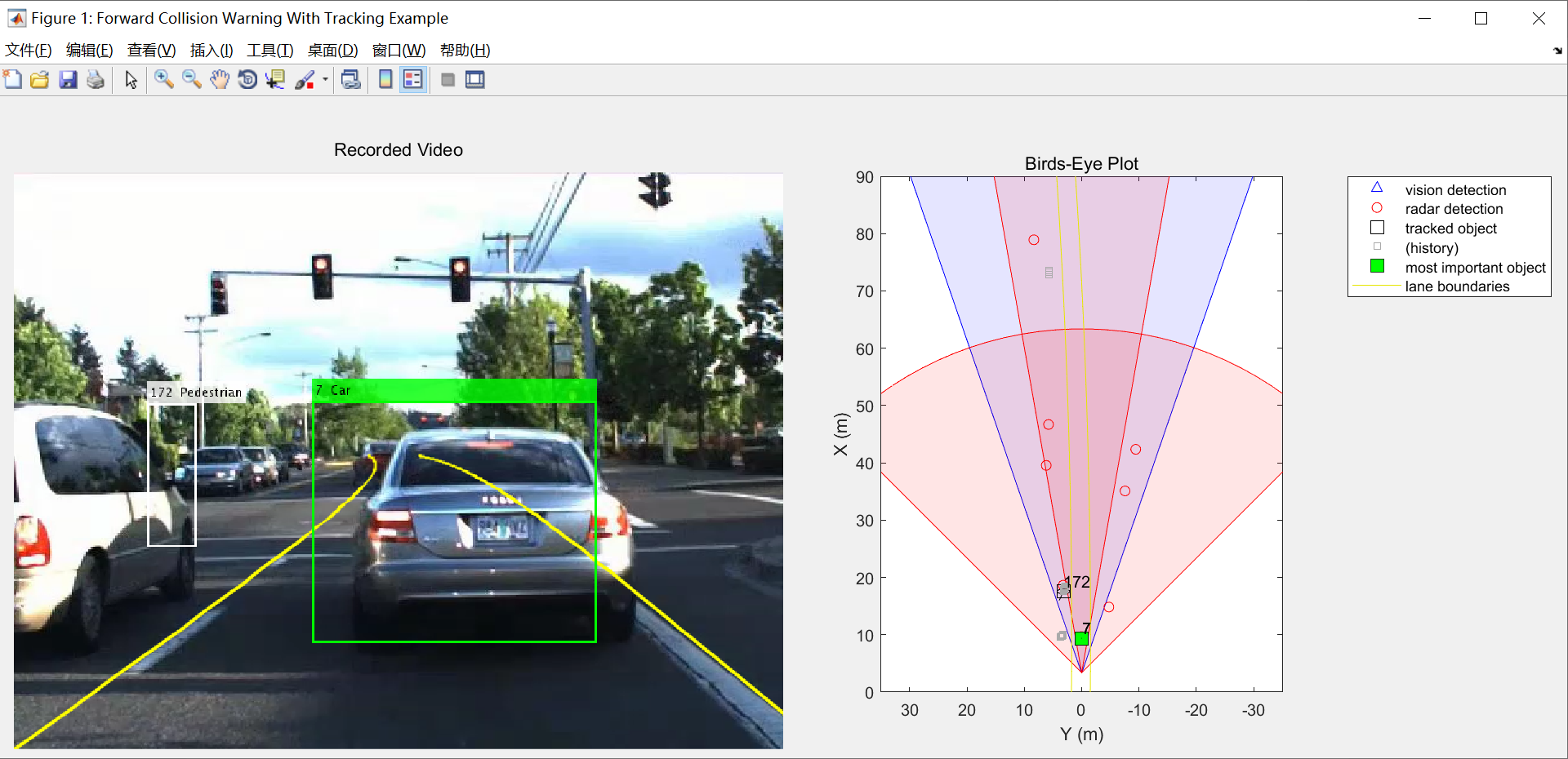
自动驾驶技术在近年来高速发展,吸引了学术界、产业界的诸多研究人员,它是一个集计算机控制技术、人工智能技术、传感探测技术等于一体的全新技术领域。自动驾驶技术自诞生以来能否对环境信息进行获取和处理是其能否落地的最关键所在。人类驾驶员是依靠人的感观能力来获取路面环境信息,依靠人类神经网络来处理信息的,而自动驾驶车辆则需要各种传感器来获取路面环境信息,利用人工智能算法来处理信息。深度学习的快速发展,为自动驾驶车辆提供了日渐完善的感知算法。随着城市机动车数量迅速增加,交通事故以及空气污染问题日益严重,针对这一现状,本文设计基于计算机视觉的辅助自动驾驶系统。辅助自动驾驶汽车对社会、驾驶员和行人均有益处,即使受其它汽车交通事故发生率的干扰,自动驾驶汽车市场份额的高速增长也会使整体交通事故发生率稳步下降。本文模拟真实道路交通场景,通过摄像头采集照片,然后通过图像处理对驾驶员驾驶过程中环境的车道线、交通信号灯和车辆进行检测和识别,最后把检测结果反馈给驾驶员,提醒驾驶员安全驾驶,达到更加节能、高效的行驶模式。
📚2 运行结果
部分代码:
% Set up the display
[videoReader, videoDisplayHandle, bepPlotters, sensor] = helperCreateFCWDemoDisplay('01_city_c2s_fcw_10s.mp4', 'SensorConfigurationData.mat');
% Read the recorded detections file
[visionObjects, radarObjects, inertialMeasurementUnit, laneReports, ...
timeStep, numSteps] = readSensorRecordingsFile('01_city_c2s_fcw_10s_sensor.mat');
% An initial ego lane is calculated. If the recorded lane information is
% invalid, define the lane boundaries as straight lines half a lane
% distance on each side of the car
laneWidth = 3.6; % meters
egoLane = struct('left', [0 0 laneWidth/2], 'right', [0 0 -laneWidth/2]);
% Prepare some time variables
time = 0; % Time since the beginning of the recording
currentStep = 0; % Current timestep
snapTime = 9.3; % The time to capture a snapshot of the display
% Initialize the tracker
[tracker, positionSelector, velocitySelector] = setupTracker();
while currentStep < numSteps && ishghandle(videoDisplayHandle)
% Update scenario counters
currentStep = currentStep + 1;
time = time + timeStep;
% Process the sensor detections as objectDetection inputs to the tracker
[detections, laneBoundaries, egoLane] = processDetections(...
visionObjects(currentStep), radarObjects(currentStep), ...
inertialMeasurementUnit(currentStep), laneReports(currentStep), ...
egoLane, time);
% Using the list of objectDetections, return the tracks, updated to time
confirmedTracks = updateTracks(tracker, detections, time);
% Find the most important object and calculate the forward collision
% warning
mostImportantObject = findMostImportantObject(confirmedTracks, egoLane, positionSelector, velocitySelector);
% Update video and birds-eye plot displays
frame = readFrame(videoReader); % Read video frame
helperUpdateFCWDemoDisplay(frame, videoDisplayHandle, bepPlotters, ...
laneBoundaries, sensor, confirmedTracks, mostImportantObject, positionSelector, ...
velocitySelector, visionObjects(currentStep), radarObjects(currentStep));
% Capture a snapshot
if time >= snapTime && time < snapTime + timeStep
snapnow;
end
end
displayEndOfDemoMessage(mfilename)
%% Create the Multi-Object Tracker
% The |multiObjectTracker| tracks the objects around the ego vehicle based
% on the object lists reported by the vision and radar sensors. By fusing
% information from both sensors, the probabilty of a false collision
% warning is reduced.
%
% The |setupTracker| function returns the |multiObjectTracker|.
% When creating a |multiObjectTracker|, consider the following:
%
% # |FilterInitializationFcn|: The likely motion and measurement models.
% In this case, the objects are expected to have a constant acceleration
% motion. Although you can configure a linear Kalman filter for this
% model, |initConstantAccelerationFilter| configures an extended Kalman
% filter. See the 'Define a Kalman filter' section.
% # |AssignmentThreshold|: How far detections can fall from tracks.
% The default value for this parameter is 30. If there are detections
% that are not assigned to tracks, but should be, increase this value. If
% there are detections that get assigned to tracks that are too far,
% decrease this value. This example uses 35.
% # |NumCoastingUpdates|: How many times a track is coasted before deletion.
% Coasting is a term used for updating the track without an assigned
% detection (predicting).
% The default value for this parameter is 5. In this case, the tracker is
% called 20 times a second and there are two sensors, so there is no need
% to modify the default.
% # |ConfirmationParameters|: The parameters for confirming a track.
% A new track is initialized with every unassigned detection. Some of
% these detections might be false, so all the tracks are initialized as
% |'Tentative'|. To confirm a track, it has to be detected at least _M_
% times in _N_ tracker updates. The choice of _M_ and _N_ depends on the
% visibility of the objects. This example uses the default of 2
% detections out of 3 updates.
%
% The outputs of |setupTracker| are:
%
% * |tracker| - The |multiObjectTracker| that is configured for this case.
% * |positionSelector| - A matrix that specifies which elements of the
% State vector are the position: |position = positionSelector * State|
% * |velocitySelector| - A matrix that specifies which elements of the
% State vector are the velocity: |velocity = velocitySelector * State|
function [tracker, positionSelector, velocitySelector] = setupTracker()
tracker = multiObjectTracker(...
'FilterInitializationFcn', @initConstantAccelerationFilter, ...
'AssignmentThreshold', 35, 'ConfirmationParameters', [2 3], ...
'NumCoastingUpdates', 5);
% The State vector is:
% In constant velocity: State = [x;vx;y;vy]
% In constant acceleration: State = [x;vx;ax;y;vy;ay]
% Define which part of the State is the position. For example:
% In constant velocity: [x;y] = [1 0 0 0; 0 0 1 0] * State
% In constant acceleration: [x;y] = [1 0 0 0 0 0; 0 0 0 1 0 0] * State
positionSelector = [1 0 0 0 0 0; 0 0 0 1 0 0];
% Define which part of the State is the velocity. For example:
% In constant velocity: [x;y] = [0 1 0 0; 0 0 0 1] * State
% In constant acceleration: [x;y] = [0 1 0 0 0 0; 0 0 0 0 1 0] * State
velocitySelector = [0 1 0 0 0 0; 0 0 0 0 1 0];
end
%% Define a Kalman Filter
% The |multiObjectTracker| defined in the previous section uses the filter
% initialization function defined in this section to create a Kalman filter
% (linear, extended, or unscented). This filter is then used for tracking
% each object around the ego vehicle.
function filter = initConstantAccelerationFilter(detection)
% This function shows how to configure a constant acceleration filter. The
% input is an objectDetection and the output is a tracking filter.
% For clarity, this function shows how to configure a trackingKF,
% trackingEKF, or trackingUKF for constant acceleration.
%
% Steps for creating a filter:
% 1. Define the motion model and state
% 2. Define the process noise
% 3. Define the measurement model
% 4. Initialize the state vector based on the measurement
% 5. Initialize the state covariance based on the measurement noise
% 6. Create the correct filter
% Step 1: Define the motion model and state
% This example uses a constant acceleration model, so:
STF = @constacc; % State-transition function, for EKF and UKF
STFJ = @constaccjac; % State-transition function Jacobian, only for EKF
% The motion model implies that the state is [x;vx;ax;y;vy;ay]
% You can also use constvel and constveljac to set up a constant
% velocity model, constturn and constturnjac to set up a constant turn
% rate model, or write your own models.
% Step 2: Define the process noise
dt = 0.05; % Known timestep size
sigma = 1; % Magnitude of the unknown acceleration change rate
% The process noise along one dimension
Q1d = [dt^4/4, dt^3/2, dt^2/2; dt^3/2, dt^2, dt; dt^2/2, dt, 1] * sigma^2;
Q = blkdiag(Q1d, Q1d); % 2-D process noise
% Step 3: Define the measurement model
MF = @fcwmeas; % Measurement function, for EKF and UKF
MJF = @fcwmeasjac; % Measurement Jacobian function, only for EKF
% Step 4: Initialize a state vector based on the measurement
% The sensors measure [x;vx;y;vy] and the constant acceleration model's
% state is [x;vx;ax;y;vy;ay], so the third and sixth elements of the
% state vector are initialized to zero.
state = [detection.Measurement(1); detection.Measurement(2); 0; detection.Measurement(3); detection.Measurement(4); 0];
% Step 5: Initialize the state covariance based on the measurement
% noise. The parts of the state that are not directly measured are
% assigned a large measurement noise value to account for that.
L = 100; % A large number relative to the measurement noise
stateCov = blkdiag(detection.MeasurementNoise(1:2,1:2), L, detection.MeasurementNoise(3:4,3:4), L);
% Step 6: Create the correct filter.
% Use 'KF' for trackingKF, 'EKF' for trackingEKF, or 'UKF' for trackingUKF
FilterType = 'EKF';
% Creating the filter:
switch FilterType
case 'EKF'
filter = trackingEKF(STF, MF, state,...
'StateCovariance', stateCov, ...
'MeasurementNoise', detection.MeasurementNoise(1:4,1:4), ...
'StateTransitionJacobianFcn', STFJ, ...
'MeasurementJacobianFcn', MJF, ...
'ProcessNoise', Q ...
);
case 'UKF'
filter = trackingUKF(STF, MF, state, ...
'StateCovariance', stateCov, ...
'MeasurementNoise', detection.MeasurementNoise(1:4,1:4), ...
'Alpha', 1e-1, ...
'ProcessNoise', Q ...
);
case 'KF' % The ConstantAcceleration model is linear and KF can be used
% Define the measurement model: measurement = H * state
% In this case:
% measurement = [x;vx;y;vy] = H * [x;vx;ax;y;vy;ay]
% So, H = [1 0 0 0 0 0; 0 1 0 0 0 0; 0 0 0 1 0 0; 0 0 0 0 1 0]
%
% Note that ProcessNoise is automatically calculated by the
% ConstantAcceleration motion model
H = [1 0 0 0 0 0; 0 1 0 0 0 0; 0 0 0 1 0 0; 0 0 0 0 1 0];
filter = trackingKF('MotionModel', '2D Constant Acceleration', ...
'MeasurementModel', H, 'State', state, ...
'MeasurementNoise', detection.MeasurementNoise(1:4,1:4), ...
'StateCovariance', stateCov);
end
end
%%% Process and Format the Detections
% The recorded information must be processed and formatted before it can be
% used by the tracker. This has the following steps:
%
% # Cleaning the radar detections from unnecessary clutter detections. The
% radar reports many objects that correspond to fixed objects, which
% include: guard-rails, the road median, traffic signs, etc. If these
% detections are used in the tracking, they create false tracks of fixed
% objects at the edges of the road and therefore must be removed before
% calling the tracker. Radar objects are considered nonclutter if they
% are either stationary in front of the car or moving in its vicinity.
% # Formatting the detections as input to the tracker, i.e., an array of
% <matlab:doc('objectDetection'), objectDetection> elements. See the
% |processVideo| and |processRadar| supporting functions at the end of
% this example.
function [detections,laneBoundaries, egoLane] = processDetections...
(visionFrame, radarFrame, IMUFrame, laneFrame, egoLane, time)
% Inputs:
% visionFrame - objects reported by the vision sensor for this time frame
% radarFrame - objects reported by the radar sensor for this time frame
% IMUFrame - inertial measurement unit data for this time frame
% laneFrame - lane reports for this time frame
% egoLane - the estimated ego lane
% time - the time corresponding to the time frame
% Remove clutter radar objects
[laneBoundaries, egoLane] = processLanes(laneFrame, egoLane);
realRadarObjects = findNonClutterRadarObjects(radarFrame.object,...
radarFrame.numObjects, IMUFrame.velocity, laneBoundaries);
% Return an empty list if no objects are reported
% Counting the total number of object
detections = {};
if (visionFrame.numObjects + numel(realRadarObjects)) == 0
return;
end
% Process the remaining radar objects
detections = processRadar(detections, realRadarObjects, time);
% Process video objects
detections = processVideo(detections, visionFrame, time);
end
%% Update the Tracker
% To update the tracker, call the |updateTracks| method with the following
% inputs:
%
% # |tracker| - The |multiObjectTracker| that was configured earlier. See
% the 'Create the Multi-Object Tracker' section.
% # |detections| - A list of |objectDetection| objects that was created by
% |processDetections|
% # |time| - The current scenario time.
%
% The output from the tracker is a |struct| array of tracks.
%%% Find the Most Important Object and Issue a Forward Collision Warning
% The most important object (MIO) is defined as the track that is in the
% ego lane and is closest in front of the car, i.e., with the smallest
% positive _x_ value. To lower the probability of false alarms, only
% confirmed tracks are considered.
%
% Once the MIO is found, the relative speed between the car and MIO is
% calculated. The relative distance and relative speed determine the
% forward collision warning. There are 3 cases of FCW:
%
% # Safe (green): There is no car in the ego lane (no MIO), the MIO is
% moving away from the car, or the distance is maintained constant.
% # Caution (yellow): The MIO is moving closer to the car, but is still at
% a distance above the FCW distance. FCW distance is calculated using the
% Euro NCAP AEB Test Protocol. Note that this distance varies with the
% relative speed between the MIO and the car, and is greater when the
% closing speed is higher.
% # Warn (red): The MIO is moving closer to the car, and its distance is
% less than the FCW distance.
%
% Euro NCAP AEB Test Protocol defines the following distance calculation:
%%
% $d_{FCW} = 1.2 * v_{rel} + \frac{v_{rel}^2}{2a_{max}}$
%
% where:
%
% $d_{FCW}$ is the forward collision warning distance.
%
% $v_{rel}$ is the relative velocity between the two vehicles.
%
% $a_{max}$ is the maximum deceleration, defined to be 40% of the gravity
% acceleration.
function mostImportantObject = findMostImportantObject(confirmedTracks,egoLane,positionSelector,velocitySelector)
% Initialize outputs and parameters
MIO = []; % By default, there is no MIO
trackID = []; % By default, there is no trackID associated with an MIO
FCW = 3; % By default, if there is no MIO, then FCW is 'safe'
threatColor = 'green'; % By default, the threat color is green
maxX = 1000; % Far enough forward so that no track is expected to exceed this distance
gAccel = 9.8; % Constant gravity acceleration, in m/s^2
maxDeceleration = 0.4 * gAccel; % Euro NCAP AEB definition
delayTime = 1.2; % Delay time for a driver before starting to break, in seconds
positions = getTrackPositions(confirmedTracks, positionSelector);
velocities = getTrackVelocities(confirmedTracks, velocitySelector);
for i = 1:numel(confirmedTracks)
x = positions(i,1);
y = positions(i,2);
relSpeed = velocities(i,1); % The relative speed between the cars, along the lane
if x < maxX && x > 0 % No point checking otherwise
yleftLane = polyval(egoLane.left, x);
yrightLane = polyval(egoLane.right, x);
if (yrightLane <= y) && (y <= yleftLane)
maxX = x;
trackID = i;
MIO = confirmedTracks(i).TrackID;
if relSpeed < 0 % Relative speed indicates object is getting closer
% Calculate expected braking distance according to
% Euro NCAP AEB Test Protocol
d = abs(relSpeed) * delayTime + relSpeed^2 / 2 / maxDeceleration;
if x <= d % 'warn'
FCW = 1;
threatColor = 'red';
else % 'caution'
FCW = 2;
threatColor = 'yellow';
end
end
end
end
end
mostImportantObject = struct('ObjectID', MIO, 'TrackIndex', trackID, 'Warning', FCW, 'ThreatColor', threatColor);
end
🎉3 参考文献
部分理论来源于网络,如有侵权请联系删除。
[1]陈佳. 自动驾驶环境感知中的目标跟踪与轨迹预测研究[D].北京科技大学,2022.DOI:10.26945/d.cnki.gbjku.2022.000276.
[2]杜丽. 面向自动驾驶的场景理解关键技术研究[D].北京邮电大学,2021.DOI:10.26969/d.cnki.gbydu.2021.000085.
[3]罗国荣,戚金凤.基于计算机视觉的自动驾驶汽车车道检测[J].北京工业职业技术学院学报,2020,19(04):34-37.


 2167
2167


 被折叠的 条评论
为什么被折叠?
被折叠的 条评论
为什么被折叠?
 到【灌水乐园】发言


