


对比【numpy】和【pytorch】程序,总结并陈述。
激活函数Sigmoid用PyTorch自带函数torch.sigmoid(),观察、总结并陈述。
激活函数Sigmoid改变为Relu,观察、总结并陈述。
损失函数MSE用PyTorch自带函数 t.nn.MSELoss()替代,观察、总结并陈述。
损失函数MSE改变为交叉熵,观察、总结并陈述。
改变步长,训练次数,观察、总结并陈述。
权值w1-w8初始值换为随机数,对比“指定权值”的结果,观察、总结并陈述。
权值w1-w8初始值换为0,观察、总结并陈述。
全面总结反向传播原理和编码实现,认真写心得体会。
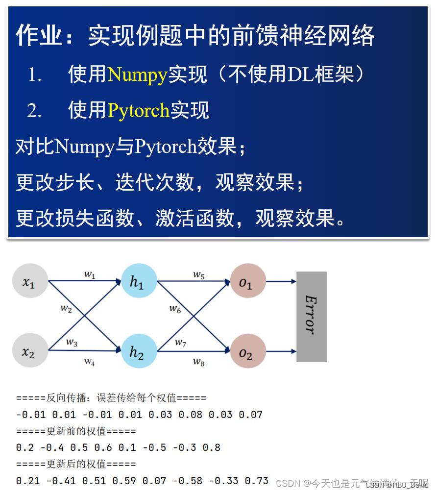
一、过程推导 - 了解BP原理和数值计算 - 手动计算,掌握细节
这两个写到一起了。
(一)、目前已知
x1=0.5 x2=0.3 y1=0.23 y2=-0.07 以及权重w1~w8
相关导的公式:
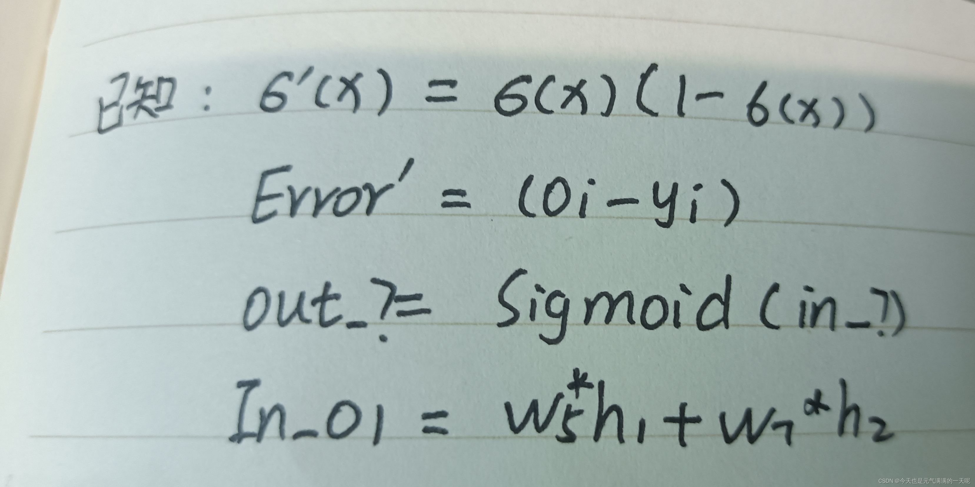
为方便计算又画了一遍图【图中变量名就是后期推导的名称】: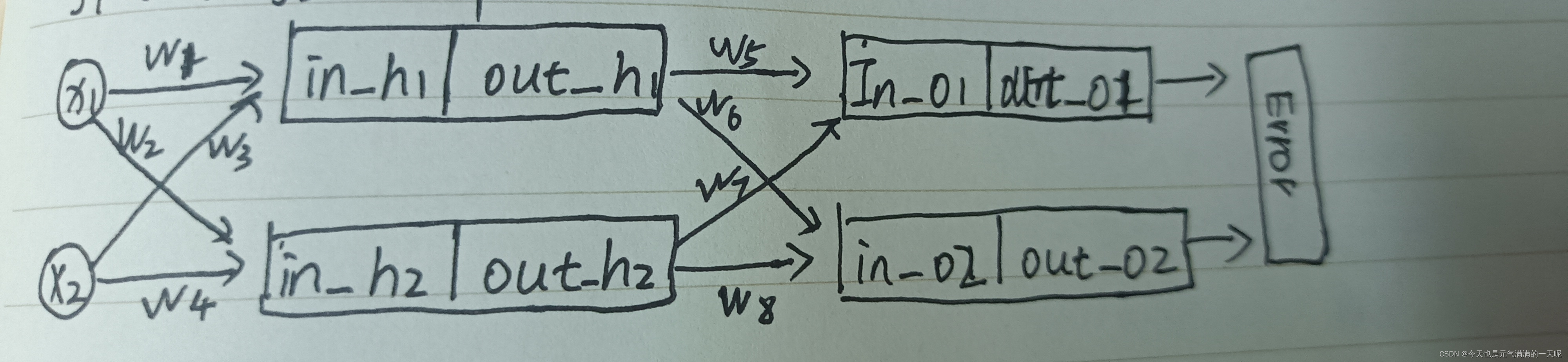
(二)、编程求解sigmoid
由于sigmoid函数手工计算比较麻烦,所以使用编程求解h1、h2和o1、o2。
(1)定义函数
import numpy as np
def sigmoid(x):
    return 1 / (1 + np.exp(-x))
(2)求解
x1=0.5
x2=0.3
y1,y2 = 0.23, -0.07
w=[0.2,-0.4,0.5,0.6,0.1,-0.5,-0.3,0.8]

#h
in_h1=x1*w[0]+x2*w[2]
in_h2=x2*w[3]+x1*w[1]
out_h1=sigmoid(in_h1)
out_h2=sigmoid(in_h2)
in_h1 = round(in_h1, 2)
in_h2 = round(in_h2, 2)
out_h1 = round(out_h1, 2)
out_h2 = round(out_h2, 2)
print('in_h1',in_h1,'in_h2',in_h2,'out_h1',out_h1,'out_h2',out_h2)

#o
in_o1=out_h1*w[4]+out_h2*w[6]
in_o2=out_h1*w[5]+out_h2*w[7]
out_o1=sigmoid(in_o1)
out_o2=sigmoid(in_o2)
in_o1 = round(in_o1, 2)
in_o2 = round(in_o2, 2)
out_o1 = round(out_o1, 2)
out_o2 = round(out_o2, 2)
print('in_o1',in_o1,'in_o2',in_o2,'out_o1',out_o1,'out_o2',out_o2)
(3)得到结果


(三)、推导

 如此,就求出了w1~w8的导
(四)、更新权重
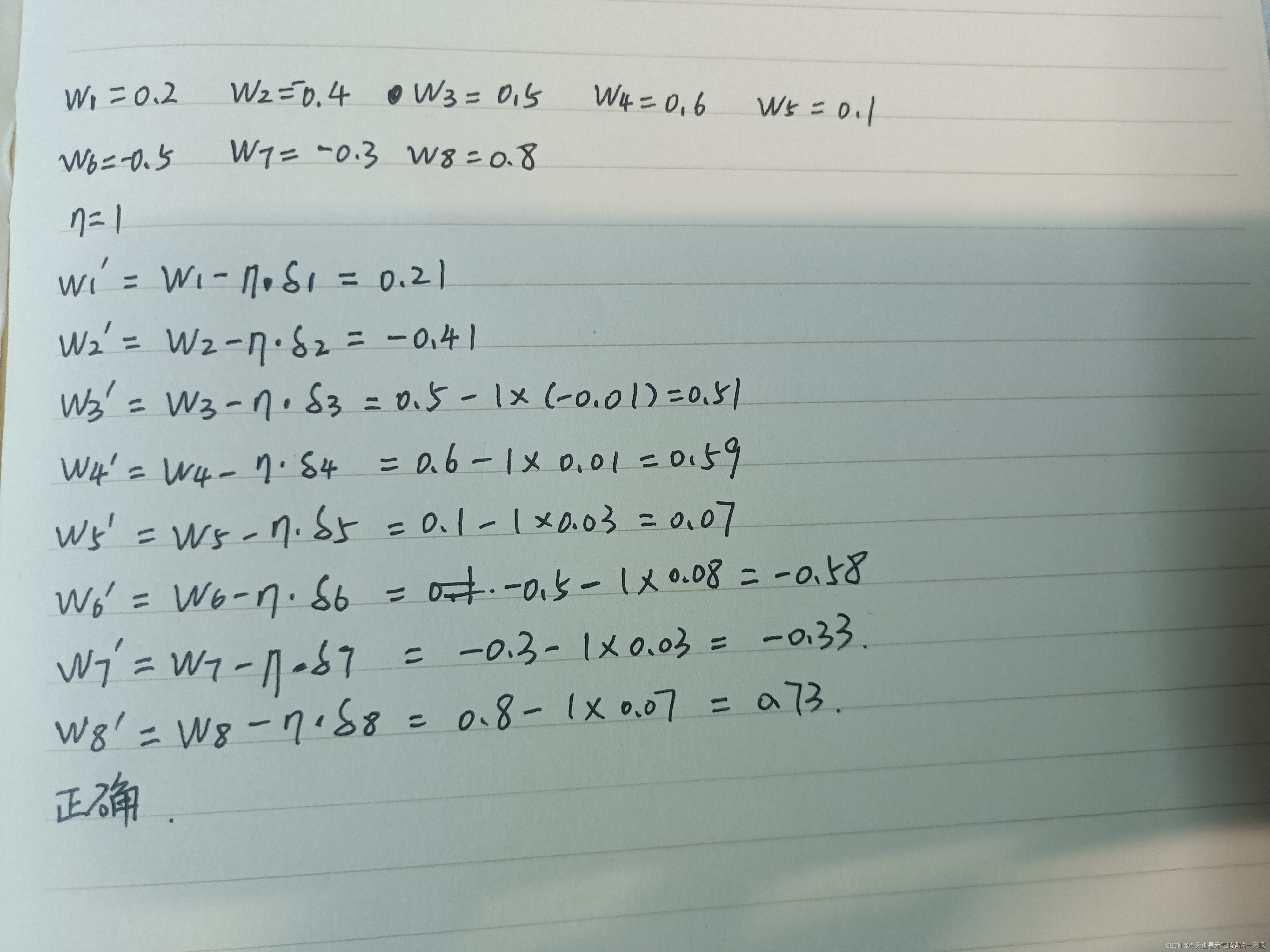
可以看到,更新后的权重与题中相同。
二、代码实现 - numpy手推 + pytorch自动
(一)、numpy完全手推
第一次写的numpy代码是直接按照前边手写公式推的,如下:
import numpy as np
def sigmoid(x):
    return 1 / (1 + np.exp(-x))
x1=0.5
x2=0.3
y1,y2 = 0.23, -0.07
w=[0.2,-0.4,0.5,0.6,0.1,-0.5,-0.3,0.8]
in_h1=x1*w[0]+x2*w[2]
in_h2=x2*w[3]+x1*w[1]
out_h1=sigmoid(in_h1)
out_h2=sigmoid(in_h2)
in_h1 = round(in_h1, 2)
in_h2 = round(in_h2, 2)
out_h1 = round(out_h1, 2)
out_h2 = round(out_h2, 2)

in_o1=out_h1*w[4]+out_h2*w[6]
in_o2=out_h1*w[5]+out_h2*w[7]
out_o1=sigmoid(in_o1)
out_o2=sigmoid(in_o2)
in_o1 = round(in_o1, 2)
in_o2 = round(in_o2, 2)
out_o1 = round(out_o1, 2)
out_o2 = round(out_o2, 2)

#反向推导
def sigmoid_dao(x):
    return x*(1-x)
def error_dao(out_o,y):
    return out_o-y
w_dao=[0]*8
w_dao[4]=error_dao(out_o1,y1)*sigmoid_dao(out_o1)*out_h1
w_dao[5]=error_dao(out_o2,y2)*sigmoid_dao(out_o2)*out_h1
w_dao[6]=error_dao(out_o1,y1)*sigmoid_dao(out_o1)*out_h2
w_dao[7]=error_dao(out_o2,y2)*sigmoid_dao(out_o2)*out_h2

H1=error_dao(out_o1,y1)*sigmoid_dao(out_o1)
H2=error_dao(out_o2,y2)*sigmoid_dao(out_o2)
w_dao[0]=(H1*w[4]+H2*w[5])*sigmoid_dao(out_h1)*x1
w_dao[1]=(H1*w[6]+H2*w[7])*sigmoid_dao(out_h2)*x1
w_dao[2]=(H1*w[4]+H2*w[5])*sigmoid_dao(out_h1)*x2
w_dao[3]=(H1*w[6]+H2*w[7])*sigmoid_dao(out_h2)*x2
H1 = round(H1, 2)
H2 = round(H2, 2)
for i in range(8):
    w_dao[i]= round(w_dao[i], 2)
for i in range(8):
    print('w_dao:',i+1,w_dao[i])

n=1
w_xin=[0]*8
for i in range(8):
    w_xin[i]=w[i]-n*w_dao[i]
    w_xin[i]=round(w_xin[i],2)
    print(i+1,w_xin[i])
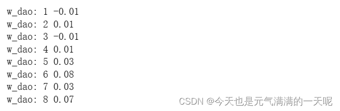
得到的结果是:
w的导:
w的更新:
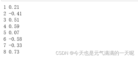
可以看到上边的两张图,与我自己手写推导的结果相同。
(二)、numpy改良
由于后边问题中,要求更改步长、迭代次数,观察效果,需要把前边的代码改良一下。
(1)封装的函数
第一部分:小函数的封装【sigmoid函数、sigmoid导的函数、error对out_o求的导、Error】
def sigmoid(x):
    return 1 / (1 + np.exp(-x))
def sigmoid_dao(x):
    return x*(1-x)
def error_dao(out_o,y):
    return out_o-y
def Error(out_o1,out_o2,y1,y2):
    error = (1 / 2) * (out_o1 - y1) ** 2 + (1 / 2) * (out_o2 - y2) ** 2
    error=round(error,2)
    return error
第二部分: 正向计算,求解out_*
#正向计算
def forward(w,x1,x2,y1,y2):

    in_h1=x1*w[0]+x2*w[2]
    in_h2=x2*w[3]+x1*w[1]
    out_h1=sigmoid(in_h1)
    out_h2=sigmoid(in_h2)

    in_h1 = round(in_h1, 2)
    in_h2 = round(in_h2, 2)
    out_h1 = round(out_h1, 2)
    out_h2 = round(out_h2, 2)
    in_o1=out_h1*w[4]+out_h2*w[6]
    in_o2=out_h1*w[5]+out_h2*w[7]
    out_o1=sigmoid(in_o1)
    out_o2=sigmoid(in_o2)
    in_o1 = round(in_o1, 2)
    in_o2 = round(in_o2, 2)
    out_o1 = round(out_o1, 2)
    out_o2 = round(out_o2, 2)

    return out_h1,out_h2,out_o1,out_o2
第三部分:反向求解w的梯度
#反向计算
def back(out_h1,out_h2,out_o1,out_o2):
    w_dao=[0]*8
    w_dao[4]=error_dao(out_o1,y1)*sigmoid_dao(out_o1)*out_h1
    w_dao[5]=error_dao(out_o2,y2)*sigmoid_dao(out_o2)*out_h1
    w_dao[6]=error_dao(out_o1,y1)*sigmoid_dao(out_o1)*out_h2
    w_dao[7]=error_dao(out_o2,y2)*sigmoid_dao(out_o2)*out_h2

    H1=error_dao(out_o1,y1)*sigmoid_dao(out_o1)
    H2=error_dao(out_o2,y2)*sigmoid_dao(out_o2)
    w_dao[0]=(H1*w[4]+H2*w[5])*sigmoid_dao(out_h1)*x1
    w_dao[1]=(H1*w[6]+H2*w[7])*sigmoid_dao(out_h2)*x1
    w_dao[2]=(H1*w[4]+H2*w[5])*sigmoid_dao(out_h1)*x2
    w_dao[3]=(H1*w[6]+H2*w[7])*sigmoid_dao(out_h2)*x2

    for i in range(8):
        w_dao[i]= round(w_dao[i], 2)
    return w_dao
第四部分:w更新
#更新权重
def updata(n,w,w_dao):
    w_xin=[0]*8
    for i in range(8):
        w_xin[i]=w[i]-n*w_dao[i]
        w_xin[i]=round(w_xin[i],2)
    return w_xin
(2)实例化
x1=0.5
x2=0.3
y1,y2 = 0.23, -0.07
w=[0.2,-0.4,0.5,0.6,0.1,-0.5,-0.3,0.8]
n=1

print('更新前的权重',w)

for i in range(51):
    out_h1,out_h2,out_o1,out_o2=forward(w,x1,x2,y1,y2)
    w_dao=back(out_h1,out_h2,out_o1,out_o2)
    w=updata(n,w,w_dao)
    error=Error(out_o1,out_o2,y1,y2)
    if i%10==0:
        print("第",i,"轮次")
        print("正向计算:",out_o1,out_o2)
        print("反向计算,得到w的导:",w_dao)
        print("损失函数(均方误差):",error)
        print("更新后的权值w",w)
(3)结果
更新五十次,得到以下结果(每十次的一次结果),并且保留两位小数
更新前的权重 [0.2, -0.4, 0.5, 0.6, 0.1, -0.5, -0.3, 0.8]
第 0 轮次
正向计算: 0.48 0.53
反向计算,得到w的导: [-0.01, 0.01, -0.01, 0.01, 0.03, 0.08, 0.03, 0.07]
损失函数(均方误差): 0.21
更新后的权值w [0.21, -0.41, 0.51, 0.59, 0.07, -0.58, -0.33, 0.73]
第 10 轮次
正向计算: 0.4 0.35
反向计算,得到w的导: [-0.02, -0.0, -0.01, -0.0, 0.02, 0.06, 0.02, 0.05]
损失函数(均方误差): 0.1
更新后的权值w [0.33, -0.45, 0.61, 0.57, -0.22, -1.27, -0.58, 0.14]
第 20 轮次
正向计算: 0.35 0.25
反向计算,得到w的导: [-0.01, -0.0, -0.01, -0.0, 0.02, 0.04, 0.01, 0.03]
损失函数(均方误差): 0.06
更新后的权值w [0.44, -0.45, 0.71, 0.57, -0.42, -1.71, -0.75, -0.22]
第 30 轮次
正向计算: 0.32 0.19
反向计算,得到w的导: [-0.01, -0.0, -0.01, -0.0, 0.01, 0.02, 0.01, 0.02]
损失函数(均方误差): 0.04
更新后的权值w [0.54, -0.45, 0.81, 0.57, -0.56, -2.0, -0.85, -0.45]
第 40 轮次
正向计算: 0.29 0.15
反向计算,得到w的导: [-0.01, -0.0, -0.0, -0.0, 0.01, 0.02, 0.01, 0.01]
损失函数(均方误差): 0.03
更新后的权值w [0.64, -0.45, 0.9, 0.57, -0.66, -2.21, -0.95, -0.64]
第 50 轮次
正向计算: 0.28 0.13
反向计算,得到w的导: [-0.01, -0.0, -0.0, -0.0, 0.01, 0.01, 0.0, 0.01]
损失函数(均方误差): 0.02
更新后的权值w [0.74, -0.45, 0.9, 0.57, -0.76, -2.37, -0.98, -0.74]
(三)、改为pytorch
(1)代码
import torch

def sigmoid(x):
    return 1 / (1 + torch.exp(-x))

def sigmoid_derivative(x):
    return x * (1 - x)

def forward(x1,x2):

    in_h1=x1*w[0]+x2*w[2]
    in_h2=x2*w[3]+x1*w[1]
    out_h1=sigmoid(in_h1)
    out_h2=sigmoid(in_h2)
    in_o1=out_h1*w[4]+out_h2*w[6]
    in_o2=out_h1*w[5]+out_h2*w[7]
    out_o1=sigmoid(in_o1)
    out_o2=sigmoid(in_o2)
    print("正向计算:h1 ,h2:",out_h1.data, out_h2.data)
    print("正向计算:o1 ,o2:",out_o1.data, out_o2.data)

    return out_o1, out_o2

def update(n, w, w_dao):
    w_updated = []
    for i in range(8):
        w_updated.append(w[i] - n * w_dao[i])
    return w_updated

def Error(x1,x2,y1,y2):
    y_pre = forward(x1,x2)  # 前向传播
    loss_mse =(1/2)*(y_pre[0]-y1)**2+(1/2)*(y_pre[1]-y2)** 2 # 考虑 : t.nn.MSELoss()
    print("损失函数(均方误差):", loss_mse.item())
    return loss_mse

# 定义x1, x2, y1, y2和初始权重w
x1 = torch.tensor([0.5])
x2 = torch.tensor([0.3])
y1 = torch.tensor([0.23])
y2 = torch.tensor([-0.07])
w = [torch.Tensor([0.2]), torch.Tensor([-0.4]), torch.Tensor([0.5]), torch.Tensor([0.6]), torch.Tensor([0.1]), torch.Tensor([-0.5]), torch.Tensor([-0.3]), torch.Tensor([0.8])]
n = 1  # 步长

for i in range(0, 8):
    w[i].requires_grad = True
    print("权值w0-w7:",w[i].data)

for j in range(51):
    print("\n=====第" + str(j+1) + "轮=====")
    L = Error(x1,x2,y1,y2)  # 前向传播
    L.backward()  # 反向传播,自动求梯度。
    print("w的梯度: ", end="  ")
    for i in range(0, 8):
        print(round(w[i].grad.item(), 2), end="  ")
    for i in range(0, 8):
        w[i].data = w[i].data-n * w[i].grad.data  # 更新权值
        w[i].grad.data.zero_()  # 注意:将w中所有梯度清零
        print("\n更新后的权值w:",w[i].data)
(2)结果
第 0 轮
损失函数(均方误差): 0.2097097933292389
-0.01  0.01  -0.01  0.01  0.03  0.08  0.03  0.07  更新后的权值w: tensor([0.2084])
更新后的权值w: tensor([-0.4126])
更新后的权值w: tensor([0.5051])
更新后的权值w: tensor([0.5924])
更新后的权值w: tensor([0.0654])
更新后的权值w: tensor([-0.5839])
更新后的权值w: tensor([-0.3305])
更新后的权值w: tensor([0.7262])

第 10 轮
损失函数(均方误差): 0.10375461727380753
-0.02  -0.0  -0.01  -0.0  0.02  0.06  0.02  0.05  更新后的权值w: tensor([0.3425])
更新后的权值w: tensor([-0.4540])
更新后的权值w: tensor([0.5855])
更新后的权值w: tensor([0.5676])
更新后的权值w: tensor([-0.2230])
更新后的权值w: tensor([-1.2686])
更新后的权值w: tensor([-0.5765])
更新后的权值w: tensor([0.1418])

第 20 轮
损失函数(均方误差): 0.05818723142147064
-0.01  -0.0  -0.01  -0.0  0.02  0.04  0.01  0.03  更新后的权值w: tensor([0.4856])
更新后的权值w: tensor([-0.4246])
更新后的权值w: tensor([0.6714])
更新后的权值w: tensor([0.5853])
更新后的权值w: tensor([-0.4255])
更新后的权值w: tensor([-1.7091])
更新后的权值w: tensor([-0.7422])
更新后的权值w: tensor([-0.2187])

第 30 轮
损失函数(均方误差): 0.03740861266851425
-0.01  -0.0  -0.01  -0.0  0.01  0.02  0.01  0.02  更新后的权值w: tensor([0.6021])
更新后的权值w: tensor([-0.3828])
更新后的权值w: tensor([0.7413])
更新后的权值w: tensor([0.6103])
更新后的权值w: tensor([-0.5658])
更新后的权值w: tensor([-2.0030])
更新后的权值w: tensor([-0.8544])
更新后的权值w: tensor([-0.4537])

第 40 轮
损失函数(均方误差): 0.026734821498394012
-0.01  -0.0  -0.0  -0.0  0.01  0.02  0.01  0.01  更新后的权值w: tensor([0.6939])
更新后的权值w: tensor([-0.3438])
更新后的权值w: tensor([0.7963])
更新后的权值w: tensor([0.6337])
更新后的权值w: tensor([-0.6630])
更新后的权值w: tensor([-2.2142])
更新后的权值w: tensor([-0.9311])
更新后的权值w: tensor([-0.6204])

第 50 轮
损失函数(均方误差): 0.02064337022602558
-0.01  -0.0  -0.0  -0.0  0.01  0.01  0.0  0.01  更新后的权值w: tensor([0.7672])
更新后的权值w: tensor([-0.3102])
更新后的权值w: tensor([0.8403])
更新后的权值w: tensor([0.6539])
更新后的权值w: tensor([-0.7309])
更新后的权值w: tensor([-2.3755])
更新后的权值w: tensor([-0.9843])
更新后的权值w: tensor([-0.7468])
三、问题解答
(1)、对比【numpy】和【pytorch】程序,总结并陈述。
其中numpy中所有函数都要自己写,但是在pytorch中可以直接调用backward函数,相对便利。但是我也遇到了问题:关于将数组转化为tensor类型的:
我开始使用的是:
w = torch.tensor([0.2000, -0.4000, 0.5000, 0.6000, 0.1000, -0.5000, -0.3000, 0.8000])
但是不对,只能使用下边这种方式,才能成功调用backward函数:
w = [torch.Tensor([0.2]), torch.Tensor([-0.4]), torch.Tensor([0.5]), torch.Tensor([0.6]), torch.Tensor([0.1]), torch.Tensor([-0.5]), torch.Tensor([-0.3]), torch.Tensor([0.8])]
还要注意:
for i in range(0, 8):
w[i].requires_grad = True
因为:“requires_grad”属性用于标记该张量是否需要计算其梯度。如果一个张量的“requires_grad”属性为True,那么PyTorch会在该张量进行操作时自动计算其梯度,并将结果存储在“grad”属性中。这个自动计算梯度的过程是由PyTorch的autograd系统完成的。
(2)激活函数Sigmoid用PyTorch自带函数torch.sigmoid(),观察、总结并陈述。
为对比sigmoid激活函数与torch自带sigmoid,代码如下:
torch中sigmoid函数:
def forward(x1,x2):
    in_h1 = w[0] * x[0] + w[2] * x[1]
    out_h1 = torch.sigmoid(in_h1)
    in_h2 = w[1] * x[0] + w[3] * x[1]
    out_h2 = torch.sigmoid(in_h2)

    in_o1 = w[4] * out_h1 + w[6] * out_h2
    out_o1 = torch.sigmoid(in_o1)
    in_o2 = w[5] * out_h1 + w[7] * out_h2
    out_o2 = torch.sigmoid(in_o2)
    return out_o1, out_o2

out_o1, out_o2=forward(x1,x2)
print(out_o1,out_o2)
sigmoid自写函数:
def sigmoid(x):
    return 1 / (1 + torch.exp(-x))
def forward(x1,x2):  # 计算图
    in_h1 = w[0] * x[0] + w[2] * x[1]
    out_h1 = sigmoid(in_h1)
    in_h2 = w[1] * x[0] + w[3] * x[1]
    out_h2 = sigmoid(in_h2)

    in_o1 = w[4] * out_h1 + w[6] * out_h2
    out_o1 = sigmoid(in_o1)
    in_o2 = w[5] * out_h1 + w[7] * out_h2
    out_o2 = sigmoid(in_o2)
    return out_o1, out_o2

out_o1, out_o2=forward(x1,x2)
print(out_o1,out_o2)
对比结果:

 可以看到结果相同,并没有明显区别。
(3)激活函数Sigmoid改变为Relu,观察、总结并陈述。
以pytorch为例,使用ReLu激活函数代码如下:
import torch

def relu(x):
    return torch.nn.functional.relu(x)

def forward(x1,x2):
    in_h1=x1*w[0]+x2*w[2]
    in_h2=x2*w[3]+x1*w[1]
    out_h1=relu(in_h1)
    out_h2=relu(in_h2)
    in_o1=out_h1*w[4]+out_h2*w[6]
    in_o2=out_h1*w[5]+out_h2*w[7]
    out_o1=relu(in_o1)
    out_o2=relu(in_o2)

    return out_o1, out_o2

def update(n, w, w_dao):
    w_updated = []
    for i in range(8):
        w_updated.append(w[i] - n * w_dao[i])
    return w_updated

def Error(x1,x2,y1,y2):
    y_pre = forward(x1,x2)  # 前向传播
    loss_mse =(1/2)*(y_pre[0]-y1)**2+(1/2)*(y_pre[1]-y2)** 2 # 考虑 : t.nn.MSELoss()
    return loss_mse

x1 = torch.tensor([0.5])
x2 = torch.tensor([0.3])
y1 = torch.tensor([0.23])
y2 = torch.tensor([-0.07])
w = [torch.Tensor([0.2]), torch.Tensor([-0.4]), torch.Tensor([0.5]), torch.Tensor([0.6]), torch.Tensor([0.1]), torch.Tensor([-0.5]), torch.Tensor([-0.3]), torch.Tensor([0.8])]
n = 1  # 步长

for i in range(0, 8):
    w[i].requires_grad = True

for j in range(1):
    L = Error(x1,x2,y1,y2)  # 前向传播
    L.backward()  # 反向传播,自动求梯度。
    if j%10==0:
        print("\n第",j,"轮")
        print("损失函数(均方误差):", L.item())
    for i in range(0, 8):
        if j%10==0:
            print(round(w[i].grad.item(), 2), end="  ")
    for i in range(0, 8):
        w[i].data = w[i].data-n * w[i].grad.data  # 更新权值
        w[i].grad.data.zero_()  # 注意:将w中所有梯度清零
        if j%10==0:
            print("更新后的权值w:",w[i].data)
对比两种激活函数结果:
sigmoid:
第 1 轮
损失函数(均方误差): 0.2097097933292389
-0.01  0.01  -0.01  0.01  0.03  0.08  0.03  0.07  更新后的权值w: tensor([0.2084])
更新后的权值w: tensor([-0.4126])
更新后的权值w: tensor([0.5051])
更新后的权值w: tensor([0.5924])
更新后的权值w: tensor([0.0654])
更新后的权值w: tensor([-0.5839])
更新后的权值w: tensor([-0.3305])
更新后的权值w: tensor([0.7262])
第 11 轮
损失函数(均方误差): 0.10375461727380753
-0.02 -0.0 -0.01 -0.0 0.02 0.06 0.02 0.05 更新后的权值w: tensor([0.3425])
更新后的权值w: tensor([-0.4540])
更新后的权值w: tensor([0.5855])
更新后的权值w: tensor([0.5676])
更新后的权值w: tensor([-0.2230])
更新后的权值w: tensor([-1.2686])
更新后的权值w: tensor([-0.5765])
更新后的权值w: tensor([0.1418])第 21 轮
损失函数(均方误差): 0.05818723142147064
-0.01 -0.0 -0.01 -0.0 0.02 0.04 0.01 0.03 更新后的权值w: tensor([0.4856])
更新后的权值w: tensor([-0.4246])
更新后的权值w: tensor([0.6714])
更新后的权值w: tensor([0.5853])
更新后的权值w: tensor([-0.4255])
更新后的权值w: tensor([-1.7091])
更新后的权值w: tensor([-0.7422])
更新后的权值w: tensor([-0.2187])ReLu:
第 1 轮
损失函数(均方误差): 0.023462500423192978
-0.01  0.0  -0.01  0.0  -0.05  0.0  -0.0  0.0  更新后的权值w: tensor([0.2103])
更新后的权值w: tensor([-0.4000])
更新后的权值w: tensor([0.5062])
更新后的权值w: tensor([0.6000])
更新后的权值w: tensor([0.1513])
更新后的权值w: tensor([-0.5000])
更新后的权值w: tensor([-0.3000])
更新后的权值w: tensor([0.8000])
第 11 轮
损失函数(均方误差): 0.0036630069371312857
-0.01  0.0  -0.01  0.0  -0.02  0.0  0.0  0.0  更新后的权值w: tensor([0.3877])
更新后的权值w: tensor([-0.4000])
更新后的权值w: tensor([0.6126])
更新后的权值w: tensor([0.6000])
更新后的权值w: tensor([0.5074])
更新后的权值w: tensor([-0.5000])
更新后的权值w: tensor([-0.3000])
更新后的权值w: tensor([0.8000])
第 21 轮
损失函数(均方误差): 0.0024535225238651037
-0.0 0.0 -0.0 0.0 -0.0 0.0 0.0 0.0 更新后的权值w: tensor([0.4266])
更新后的权值w: tensor([-0.4000])
更新后的权值w: tensor([0.6360])
更新后的权值w: tensor([0.6000])
更新后的权值w: tensor([0.5644])
更新后的权值w: tensor([-0.5000])
更新后的权值w: tensor([-0.3000])
更新后的权值w: tensor([0.8000])对比两组结果,可以发现ReLu的计算效率比sigmoid效率高【均方误差下降的快】,他的收敛速度也比较快。
同时搜集资料得知:当输入值为负时,ReLU输出为0,激活函数非常简单和稀疏。相比之下,Sigmoid函数在所有输入值上都有一个非零输出。这种稀疏性可以减少神经网络中的冗余和过拟合现象。
(4)损失函数MSE用PyTorch自带函数 t.nn.MSELoss()替代,观察、总结并陈述。
使用函数t.nn.MSELoss()代码如下:
import torch

def sigmoid(x):
    return 1 / (1 + torch.exp(-x))

def forward(x1,x2):

    in_h1=x1*w[0]+x2*w[2]
    in_h2=x2*w[3]+x1*w[1]
    out_h1=sigmoid(in_h1)
    out_h2=sigmoid(in_h2)
    in_o1=out_h1*w[4]+out_h2*w[6]
    in_o2=out_h1*w[5]+out_h2*w[7]
    out_o1=sigmoid(in_o1)
    out_o2=sigmoid(in_o2)

    return out_o1, out_o2

def update(n, w, w_dao):
    w_updated = []
    for i in range(8):
        w_updated.append(w[i] - n * w_dao[i])
    return w_updated
def Error(x1, x2, y1, y2):
    y_pre= forward(x1, x2)
    mse = torch.nn.MSELoss()
    loss_mse =mse(y_pre[0],y1) + mse(y_pre[1],y2)
    return loss_mse


# 定义x1, x2, y1, y2和初始权重w
x1 = torch.tensor([0.5])
x2 = torch.tensor([0.3])
y1 = torch.tensor([0.23])
y2 = torch.tensor([-0.07])
w = [torch.Tensor([0.2]), torch.Tensor([-0.4]), torch.Tensor([0.5]), torch.Tensor([0.6]), torch.Tensor([0.1]), torch.Tensor([-0.5]), torch.Tensor([-0.3]), torch.Tensor([0.8])]
n = 1  # 步长

for i in range(0, 8):
    w[i].requires_grad = True

for j in range(1001):
    L = Error(x1,x2,y1,y2)  # 前向传播
    L.backward()  # 反向传播,自动求梯度。
    if j%10==0:
        print("\n第",j+1,"轮")
        print("损失函数(均方误差):", L.item())
    for i in range(0, 8):
        if j%10==0:
            print(round(w[i].grad.item(), 2), end="  ")
    for i in range(0, 8):
        w[i].data = w[i].data-n * w[i].grad.data  # 更新权值
        w[i].grad.data.zero_()  # 注意:将w中所有梯度清零
        if j%10==0:
            print("更新后的权值w:",w[i].data)
对比手写与torch自带函数:
手写MSE:
第 1 轮
损失函数(均方误差): 0.2097097933292389
-0.01  0.01  -0.01  0.01  0.03  0.08  0.03  0.07  更新后的权值w: tensor([0.2084])
更新后的权值w: tensor([-0.4126])
更新后的权值w: tensor([0.5051])
更新后的权值w: tensor([0.5924])
更新后的权值w: tensor([0.0654])
更新后的权值w: tensor([-0.5839])
更新后的权值w: tensor([-0.3305])
更新后的权值w: tensor([0.7262])
第 51 轮
损失函数(均方误差): 0.02064337022602558
-0.01  -0.0  -0.0  -0.0  0.01  0.01  0.0  0.01  更新后的权值w: tensor([0.7672])
更新后的权值w: tensor([-0.3102])
更新后的权值w: tensor([0.8403])
更新后的权值w: tensor([0.6539])
更新后的权值w: tensor([-0.7309])
更新后的权值w: tensor([-2.3755])
更新后的权值w: tensor([-0.9843])
更新后的权值w: tensor([-0.7468])
第 101 轮
损失函数(均方误差): 0.010253453627228737
-0.0 -0.0 -0.0 -0.0 0.0 0.01 0.0 0.01 更新后的权值w: tensor([0.9896])
更新后的权值w: tensor([-0.2022])
更新后的权值w: tensor([0.9738])
更新后的权值w: tensor([0.7187])
更新后的权值w: tensor([-0.8637])
更新后的权值w: tensor([-2.8525])
更新后的权值w: tensor([-1.0873])
更新后的权值w: tensor([-1.1163])t.nn.MSELoss():
第 1 轮
损失函数(均方误差): 0.4194195866584778
-0.02 0.03 -0.01 0.02 0.07 0.17 0.06 0.15 更新后的权值w: tensor([0.2168])
更新后的权值w: tensor([-0.4252])
更新后的权值w: tensor([0.5101])
更新后的权值w: tensor([0.5849])
更新后的权值w: tensor([0.0307])
更新后的权值w: tensor([-0.6677])
更新后的权值w: tensor([-0.3610])
更新后的权值w: tensor([0.6523])第 51 轮
损失函数(均方误差): 0.020327573642134666
-0.01 -0.0 -0.0 -0.0 0.0 0.01 0.0 0.01 更新后的权值w: tensor([0.9895])
更新后的权值w: tensor([-0.2069])
更新后的权值w: tensor([0.9737])
更新后的权值w: tensor([0.7159])
更新后的权值w: tensor([-0.8678])
更新后的权值w: tensor([-2.8686])
更新后的权值w: tensor([-1.0913])
更新后的权值w: tensor([-1.1305])第 101 轮
损失函数(均方误差): 0.012286863289773464
-0.0 -0.0 -0.0 -0.0 -0.0 0.01 -0.0 0.0 更新后的权值w: tensor([1.1914])
更新后的权值w: tensor([-0.1058])
更新后的权值w: tensor([1.0948])
更新后的权值w: tensor([0.7765])
更新后的权值w: tensor([-0.8710])
更新后的权值w: tensor([-3.3064])
更新后的权值w: tensor([-1.0937])
更新后的权值w: tensor([-1.4652])可以看到在到达100轮次后,手写的MSE值小于torch自带MSE值,可知手写情况比自带情况的收敛效果好。
(5)损失函数MSE改变为交叉熵,观察、总结并陈述。
交叉熵函数代码【其他地方不变】:
def Error(x1, x2, y1, y2):
y_pre = forward(x1, x2) # 前向传播
# 创建交叉熵损失函数
loss = nn.CrossEntropyLoss()
# 将预测结果和目标标签叠加在一起
y_pred = torch.stack([y_pre[0], y_pre[1]], dim=1)
y = torch.stack([y1, y2], dim=1)
# 计算交叉熵损失
loss_ce = loss(y_pred, y)
return loss_ce得到结果:
第 1 轮
损失函数(均方误差): 0.11871970444917679
-0.0 0.01 -0.0 0.0 -0.02 0.02 -0.02 0.02 更新后的权值w: tensor([0.2028])
更新后的权值w: tensor([-0.4052])
更新后的权值w: tensor([0.5017])
更新后的权值w: tensor([0.5969])
更新后的权值w: tensor([0.1213])
更新后的权值w: tensor([-0.5213])
更新后的权值w: tensor([-0.2812])
更新后的权值w: tensor([0.7812])第 51 轮
损失函数(均方误差): 0.05054658651351929
-0.01 -0.0 -0.0 -0.0 -0.02 0.02 -0.01 0.01 更新后的权值w: tensor([0.5215])
更新后的权值w: tensor([-0.4611])
更新后的权值w: tensor([0.6929])
更新后的权值w: tensor([0.5633])
更新后的权值w: tensor([1.0931])
更新后的权值w: tensor([-1.4937])
更新后的权值w: tensor([0.5264])
更新后的权值w: tensor([-0.0268])第 101 轮
损失函数(均方误差): 0.015986934304237366
-0.01 -0.0 -0.0 -0.0 -0.01 0.01 -0.01 0.01 更新后的权值w: tensor([0.9094])
更新后的权值w: tensor([-0.3223])
更新后的权值w: tensor([0.9257])
更新后的权值w: tensor([0.6466])
更新后的权值w: tensor([1.7698])
更新后的权值w: tensor([-2.1666])
更新后的权值w: tensor([1.0463])
更新后的权值w: tensor([-0.5439])可以发现,与自带MSE相比,交叉熵损失函数在第100轮次的梯度下降较慢。
可以知道交叉熵的梯度下降速率没有MSE快。同时在本次实验中,我们关注的是预测值与真实值之间的差异,想要降低这差值。而交叉熵关注的是概率的差异更敏感,它更加关注样本的分类错误程度。
在以前的学习过程中,知道MSE适用于回归任务,交叉熵适用于分类任务。
(6)改变步长,训练次数,观察、总结并陈述。
在前边代码中改变训练次数,可以看到,训练次数越多,梯度越接近于0,损失值越小,神经网络效果越好。
改变步长:
n=1:
第 1 轮
损失函数(均方误差): 0.2097097933292389
-0.01 0.01 -0.01 0.01 0.03 0.08 0.03 0.07 更新后的权值w: tensor([0.2084])
更新后的权值w: tensor([-0.4126])
更新后的权值w: tensor([0.5051])
更新后的权值w: tensor([0.5924])
更新后的权值w: tensor([0.0654])
更新后的权值w: tensor([-0.5839])
更新后的权值w: tensor([-0.3305])
更新后的权值w: tensor([0.7262])
第 51 轮
损失函数(均方误差): 0.02064337022602558
-0.01 -0.0 -0.0 -0.0 0.01 0.01 0.0 0.01 更新后的权值w: tensor([0.7672])
更新后的权值w: tensor([-0.3102])
更新后的权值w: tensor([0.8403])
更新后的权值w: tensor([0.6539])
更新后的权值w: tensor([-0.7309])
更新后的权值w: tensor([-2.3755])
更新后的权值w: tensor([-0.9843])
更新后的权值w: tensor([-0.7468])
第 101 轮
损失函数(均方误差): 0.010253453627228737
-0.0  -0.0  -0.0  -0.0  0.0  0.01  0.0  0.01  更新后的权值w: tensor([0.9896])
更新后的权值w: tensor([-0.2022])
更新后的权值w: tensor([0.9738])
更新后的权值w: tensor([0.7187])
更新后的权值w: tensor([-0.8637])
更新后的权值w: tensor([-2.8525])
更新后的权值w: tensor([-1.0873])
更新后的权值w: tensor([-1.1163])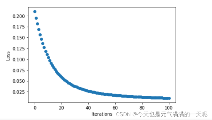
n=0.1:
第 1 轮
损失函数(均方误差): 0.2097097933292389
-0.01  0.01  -0.01  0.01  0.03  0.08  0.03  0.07  更新后的权值w: tensor([0.2008])
更新后的权值w: tensor([-0.4013])
更新后的权值w: tensor([0.5005])
更新后的权值w: tensor([0.5992])
更新后的权值w: tensor([0.0965])
更新后的权值w: tensor([-0.5084])
更新后的权值w: tensor([-0.3030])
更新后的权值w: tensor([0.7926])

第 51 轮
损失函数(均方误差): 0.1468939185142517
-0.01  0.0  -0.01  0.0  0.03  0.07  0.03  0.06  更新后的权值w: tensor([0.2584])
更新后的权值w: tensor([-0.4417])
更新后的权值w: tensor([0.5350])
更新后的权值w: tensor([0.5750])
更新后的权值w: tensor([-0.0627])
更新后的权值w: tensor([-0.8937])
更新后的权值w: tensor([-0.4411])
更新后的权值w: tensor([0.4587])

第 101 轮
损失函数(均方误差): 0.10485432296991348
-0.02  -0.0  -0.01  -0.0  0.02  0.06  0.02  0.05  更新后的权值w: tensor([0.3317])
更新后的权值w: tensor([-0.4496])
更新后的权值w: tensor([0.5790])
更新后的权值w: tensor([0.5702])
更新后的权值w: tensor([-0.1973])
更新后的权值w: tensor([-1.2086])
更新后的权值w: tensor([-0.5545])
更新后的权值w: tensor([0.1932])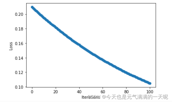
n=10:
第 1 轮
损失函数(均方误差): 0.2097097933292389
-0.01  0.01  -0.01  0.01  0.03  0.08  0.03  0.07  更新后的权值w: tensor([0.2842])
更新后的权值w: tensor([-0.5261])
更新后的权值w: tensor([0.5505])
更新后的权值w: tensor([0.5244])
更新后的权值w: tensor([-0.2463])
更新后的权值w: tensor([-1.3387])
更新后的权值w: tensor([-0.6049])
更新后的权值w: tensor([0.0616])


第 51 轮
损失函数(均方误差): 0.003888471983373165
-0.0  -0.0  -0.0  -0.0  -0.0  0.0  -0.0  0.0  更新后的权值w: tensor([1.4146])
更新后的权值w: tensor([-0.0209])
更新后的权值w: tensor([1.2287])
更新后的权值w: tensor([0.8275])
更新后的权值w: tensor([-0.8256])
更新后的权值w: tensor([-3.9177])
更新后的权值w: tensor([-1.0687])
更新后的权值w: tensor([-1.9406])

第 101 轮
损失函数(均方误差): 0.003177047474309802
-0.0  -0.0  -0.0  -0.0  -0.0  0.0  -0.0  0.0  更新后的权值w: tensor([1.6124])
更新后的权值w: tensor([0.1093])
更新后的权值w: tensor([1.3474])
更新后的权值w: tensor([0.9056])
更新后的权值w: tensor([-0.7873])
更新后的权值w: tensor([-4.3226])
更新后的权值w: tensor([-1.0398])
更新后的权值w: tensor([-2.2449])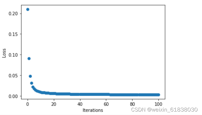
我将n=1,n=0.1,n=10分别对比输出结果与点图可以看到:当n=0.1时梯度下降速度、收敛速度太慢,但是n=10时在15轮次左右的时候梯度都已经下降到0,速度太快,不便于观察。
由此可知:将步长适当调大可以提高梯度下降速度。
(7)权值w1-w8初始值换为随机数,对比“指定权值”的结果,观察、总结并陈述。
使用以下代码初始化:
w = [torch.randn(1) for _ in range(8)]
print("随机初始化的 w:", w)
其中随机化后的w为:
随机初始化的 w: [tensor([0.5343]), tensor([-0.0909]), tensor([0.0911]), tensor([0.6306]), tensor([1.5516]), tensor([0.0103]), tensor([-0.0712]), tensor([-0.1518])]得到的结果为:
0.02  -0.0  0.01  -0.0  0.06  0.08  0.05  0.07
第 1 轮
损失函数(均方误差): 0.2627074718475342
更新后的权值w: tensor([0.5154])
更新后的权值w: tensor([-0.0874])
更新后的权值w: tensor([0.0797])
更新后的权值w: tensor([0.6327])
更新后的权值w: tensor([1.4951])
更新后的权值w: tensor([-0.0686])
更新后的权值w: tensor([-0.1241])
更新后的权值w: tensor([-0.2255])

-0.0  -0.01  -0.0  -0.0  0.01  0.01  0.01  0.01
第 51 轮
损失函数(均方误差): 0.020640043541789055
更新后的权值w: tensor([0.5296])
更新后的权值w: tensor([0.4536])
更新后的权值w: tensor([0.0882])
更新后的权值w: tensor([0.9573])
更新后的权值w: tensor([0.1301])
更新后的权值w: tensor([-1.5691])
更新后的权值w: tensor([-1.5129])
更新后的权值w: tensor([-1.7508])

-0.0  -0.0  -0.0  -0.0  0.0  0.01  0.0  0.01
第 101 轮
损失函数(均方误差): 0.00984925590455532
更新后的权值w: tensor([0.6697])
更新后的权值w: tensor([0.6586])
更新后的权值w: tensor([0.1723])
更新后的权值w: tensor([1.0803])
更新后的权值w: tensor([-0.0452])
更新后的权值w: tensor([-1.9563])
更新后的权值w: tensor([-1.7057])
更新后的权值w: tensor([-2.1770])
可以看到,初始权值对对权值w收敛影响不大,只会影响收敛的速度。
(8)权值w1-w8初始值换为0,观察、总结并陈述。
w = [torch.zeros(1) for i in range(8)]得到结果为:
0.0  0.0  0.0  0.0  0.03  0.07  0.03  0.07
第 1 轮
损失函数(均方误差): 0.1988999992609024
更新后的权值w: tensor([0.])
更新后的权值w: tensor([0.])
更新后的权值w: tensor([0.])
更新后的权值w: tensor([0.])
更新后的权值w: tensor([-0.0337])
更新后的权值w: tensor([-0.0712])
更新后的权值w: tensor([-0.0337])
更新后的权值w: tensor([-0.0712])

-0.01  -0.01  -0.0  -0.0  0.01  0.01  0.01  0.01
第 51 轮
损失函数(均方误差): 0.022186635062098503
更新后的权值w: tensor([0.3932])
更新后的权值w: tensor([0.3932])
更新后的权值w: tensor([0.2359])
更新后的权值w: tensor([0.2359])
更新后的权值w: tensor([-0.8327])
更新后的权值w: tensor([-1.6622])
更新后的权值w: tensor([-0.8327])
更新后的权值w: tensor([-1.6622])

-0.0  -0.0  -0.0  -0.0  0.0  0.01  0.0  0.01
第 101 轮
损失函数(均方误差): 0.010592692531645298
更新后的权值w: tensor([0.5907])
更新后的权值w: tensor([0.5907])
更新后的权值w: tensor([0.3544])
更新后的权值w: tensor([0.3544])
更新后的权值w: tensor([-0.9696])
更新后的权值w: tensor([-2.1009])
更新后的权值w: tensor([-0.9696])
更新后的权值w: tensor([-2.1009])
可以发现,类似w权值随机化,对神经网络的收敛结果没影响,只影响收敛速度。
(9)全面总结反向传播原理和编码实现,认真写心得体会。
1)在写numpy代码实现时,很麻烦,因为每一个函数都要自己手写实现;这时候也比较理解为什么做神经网络要使用pytorch了,因为torch里边有现成的函数,比较方便。
2)在手写求导的过程中,感觉不是很难,主要是要理清每个权值求解导数的公式。
3)numpy转为tensor过程中遇到了很多问题,比如转换,前边提到了:
发现pytorch对tensor的格式要求很严【一直报错】,还有在用ReLu时,看到学长【NNDL 作业3:分别使用numpy和pytorch实现FNN例题_。没有用n,nly,kkn3_笼子里的薛定谔的博客-CSDN博客】遇到的问题(我没想到那种错误写法,不过也长知识了):错误写法如下:
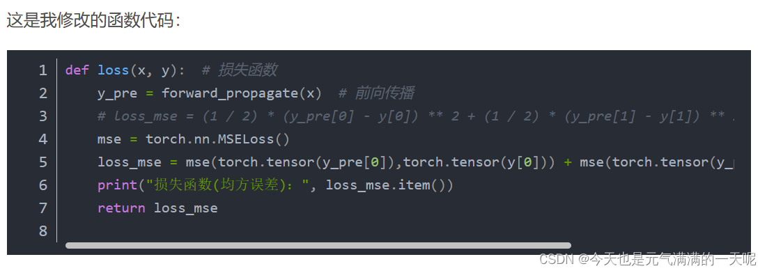
正确的是:
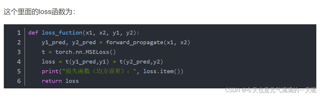
错误原因是因为y1_pred和y1本身是tensor类型的,不用再使用torch.tensor()。
其实我还是不太理解,tensor类型的数据再使用torch.tensor转出的不是tensor类型吗?为什么会报错呢?
3)在问题解答中,感觉学习到了很多:在以后的神经网络学习中,感到激活函数效果不好时,考虑更换别的激活函数;还有损失函数。
4)在多次改变权值初始值后 可以发现初始权值对对权值w收敛影响不大,只会影响收敛的速度。
5)适当的调整步长可以加快收敛速度,但是不能过大,会使得变化过大不方便观察,也可能结果不再收敛。


 526
526


 被折叠的 条评论
为什么被折叠?
被折叠的 条评论
为什么被折叠?
 到【灌水乐园】发言


