


一、实验目的
支持向量机(Support Vector Machine,SVM)是一种经典的机器学习算法,用于分类和回归任务。本实验利用机器学习算法构建支持向量机模型,实现对数据集的分类:
- 根鸢尾花数据集包含了三种不同品种的鸢尾花(山鸢尾、变色鸢尾和维吉尼亚鸢尾)的样本,每个样本有四个特征:花萼长度、花萼宽度、花瓣长度和花瓣宽度。每个样本都被标记为属于三个种类中的一个,属于一个三分类问题。
- 红酒数据集包含了三种不同品种的红酒,每个样本有十三个特征,也属于一种三分类问题。
二、实验仪器设备及软件
软件使用Google Cloaboratory的Jupyter笔记,硬件计算单元NAVIDA T4云GPU,编程语言Python。
三、实验原理
支持向量机的目标是找到一个最优的超平面,将数据集分隔成不同的类别。在二分类问题中,这个超平面被称为决策边界。在多分类问题中,支持向量机使用一对一(One-vs-One)或一对多(One-vs-Rest)的方法来处理。
四、实验步骤及程序源码
1、实验步骤
- 加载数据集并进行预处理:加载鸢尾花数据集,将数据集分割成训练集和测试集。
- 特征缩放:对特征进行标准化或归一化处理,确保不同特征的尺度一致。
- 使用支持向量机模型:选择合适的支持向量机分类器,如线性SVM或核SVM,并使用训练集对模型进行训练。
- 模型评估:使用测试集对模型进行评估,计算分类准确率等指标。
2、程序源码
(1)iris数据集实验
from google.colab import drive
drive.mount('/content/drive')
gpu_info = !nvidia-smi
gpu_info = '\n'.join(gpu_info)
if gpu_info.find('failed') >= 0:
print('Not connected to a GPU')
else:
print(gpu_info)#import xlrd
import array
import pandas as pd
import numpy as np
from matplotlib import colors
from sklearn import svm
from sklearn.svm import SVC
from sklearn import model_selection
import matplotlib.pyplot as plt
import matplotlib as mpl
#import openpyxldata_path = '/content/drive/MyDrive/大数据与信息融合实验/svm支持向量机分类/iris.xlsx' #获取数据集数据,并转换为二维数组
data = pd.read_excel(data_path,header=None)
data=data.values
print(data)
print(data.shape)#data为二维数组,data.shape=(150, 5)
#数据分割
x, y = np.split(data,(4,),axis=1)#data要切分的数组,()沿轴切分的位置,第5列开始往后为y,anxis=1代表纵向分割,按列分割
x = x[:, 0:2]
#第一个逗号之前表示行,只有冒号表示所有行,第二个冒号0:2表是0,1两列
#在X中我们取前两列作为特征,为了后面的可视化,原始的四维不好画图。x[:,0:4]代表第一维(行)全取,第二维(列)取0~2
x_train,x_test,y_train,y_test=model_selection.train_test_split(x,y,random_state=1,test_size=0.3)
#所要划分的样本特征集,所要划分的样本结果,随机数种子确保产生的随机数组相同,测试样本占比
print(x_train.shape,y_train.shape)
print(x_test.shape,y_test.shape)#**********************SVM分类器构建*************************
def classifier():
#clf = svm.SVC(C=1,kernel='rbf', gamma=50,decision_function_shape='ovr')
#clf = svm.SVC(C=1,kernel='linear',decision_function_shape='ovr')
#clf = svm.SVC(C=1,kernel='rbf',gamma='auto',decision_function_shape='ovo')#0.0001<gamma<10,0.1<C<10
clf=svm.SVC(C=7.589015815327976,kernel='rbf',gamma=0.26944843502007887,decision_function_shape='ovr')
return clf# 2.定义模型:SVM模型定义
clf = classifier()y_train.ravel()#ravel()扁平化,将原来的二维数组转换为一维数组#***********************训练模型*****************************
def train(clf,x_train,y_train):
clf.fit(x_train, #训练集特征向量,fit表示输入数据开始拟合
y_train.ravel()) #训练集目标值 ravel()扁平化,将原来的二维数组转换为一维数组# 3.训练SVM模型
train(clf,x_train,y_train)#**************并判断a b是否相等,计算acc的均值*************
def show_accuracy(a, b, tip):
acc = a.ravel() == b.ravel()
print('%s Accuracy:%.3f' %(tip, np.mean(acc)))def print_accuracy(clf,x_train,y_train,x_test,y_test):
#分别打印训练集和测试集的准确率 score(x_train,y_train):表示输出x_train,y_train在模型上的准确率
print('trianing prediction:%.3f' %(clf.score(x_train, y_train)))
print('test data prediction:%.3f' %(clf.score(x_test, y_test)))
#原始结果与预测结果进行对比 predict()表示对x_train样本进行预测,返回样本类别
show_accuracy(clf.predict(x_train), y_train, 'traing data')
show_accuracy(clf.predict(x_test), y_test, 'testing data')
#计算决策函数的值,表示x到各分割平面的距离,3类,所以有3个决策函数,不同的多类情况有不同的决策函数?
print('decision_function:\n', clf.decision_function(x_train))# 4.模型评估
print_accuracy(clf,x_train,y_train,x_test,y_test)(2)wine数据集实验
修改部分程序:
wine_path = '/content/drive/MyDrive/大数据与信息融合实验/svm支持向量机分类/wine.xlsx'
wine = pd.read_excel(wine_path,header=None)
wine=wine.values
print(wine)
print(wine.shape)
#数据分割
yy,x = np.split(wine,(1,),axis=1)#第一列类标yy,后面13列特征为x
print(yy.shape,x.shape)
x_train,x_test,y_train,y_test=model_selection.train_test_split(x,yy,random_state=1,test_size=0.3)
print(x_train.shape,y_train.shape)
print(x_test.shape,y_test.shape)#**********************SVM分类器构建*************************
def classifier():
#clf = svm.SVC(C=1,kernel='rbf', gamma=50,decision_function_shape='ovr')
#clf = svm.SVC(C=1,kernel='linear',decision_function_shape='ovr')
clf = svm.SVC(C=8,kernel='linear',gamma=10,decision_function_shape='ovr')
#clf = svm.SVC(C=100,kernel='rbf',gamma=0.0001,decision_function_shape='ovr')#0.0001<gamma<10,0.1<C<10
return clf五、实验结果与分析
1、实验结果
(1)iris数据集结果
调整SVC不同参数时可以获得不同准确度的模型:
clf = svm.SVC(C=1,kernel='rbf', gamma=50,decision_function_shape='ovr') 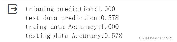
clf = svm.SVC(C=1,kernel='rbf',gamma='auto',decision_function_shape='ovo')#0.0001<gamma<10,0.1<C<10
clf = svm.SVC(C=1,kernel='linear',decision_function_shape='ovr')
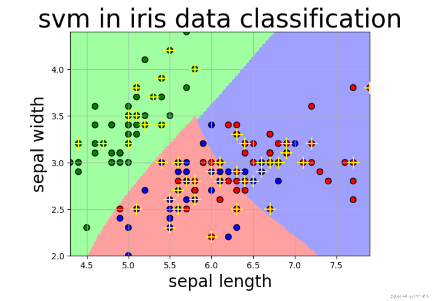
选取前两列特征,进行可视化查看数据:
def draw(clf, x):
    iris_feature = 'sepal length', 'sepal width', 'petal lenght', 'petal width'
    # 开始画图
    x1_min, x1_max = x[:, 0].min(), x[:, 0].max()               #第0列的范围
    x2_min, x2_max = x[:, 1].min(), x[:, 1].max()               #第1列的范围
    x1, x2 = np.mgrid[x1_min:x1_max:200j, x2_min:x2_max:200j]   #生成网格采样点 开始坐标:结束坐标(不包括):步长
    #flat将二维数组转换成1个1维的迭代器,然后把x1和x2的所有可能值给匹配成为样本点
    grid_test = np.stack((x1.flat, x2.flat), axis=1)            #stack():沿着新的轴加入一系列数组,竖着(按列)增加两个数组,grid_test的shape:(40000, 2)
    print('grid_test:\n', grid_test)
    # 输出样本到决策面的距离
    z = clf.decision_function(grid_test)
    print('the distance to decision plane:\n', z)

    grid_hat = clf.predict(grid_test)                           # 预测分类值 得到【0,0.。。。2,2,2】
    print('grid_hat:\n', grid_hat)
    grid_hat = grid_hat.reshape(x1.shape)                       # reshape grid_hat和x1形状一致
                                                                #若3*3矩阵e,则e.shape()为3*3,表示3行3列
 	#light是网格测试点的配色,相当于背景
    #dark是样本点的配色
    cm_light = mpl.colors.ListedColormap(['#A0FFA0', '#FFA0A0', '#A0A0FF'])
    cm_dark = mpl.colors.ListedColormap(['g', 'b', 'r'])
     #画出所有网格样本点被判断为的分类,作为背景
    plt.pcolormesh(x1, x2, grid_hat, cmap=cm_light)                                   # pcolormesh(x,y,z,cmap)这里参数代入
                                                                                      # x1,x2,grid_hat,cmap=cm_light绘制的是背景。
    #squeeze()把y的个数为1的维度去掉,也就是变成一维。
    plt.scatter(x[:, 0], x[:, 1], c=np.squeeze(y), edgecolor='k', s=50, cmap=cm_dark) # 样本点
    plt.scatter(x_test[:, 0], x_test[:, 1], s=200, facecolor='yellow', zorder=10, marker='+')       # 测试点
    plt.xlabel(iris_feature[0], fontsize=20)
    plt.ylabel(iris_feature[1], fontsize=20)
    plt.xlim(x1_min, x1_max)
    plt.ylim(x2_min, x2_max)
    plt.title('svm in iris data classification', fontsize=30)
    plt.grid()
plt.show() 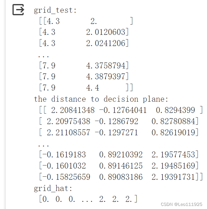
(2)wine数据集结果
调整SVC不同参数时可以获得不同准确度的模型
clf = svm.SVC(C=1,kernel='rbf', gamma=50,decision_function_shape='ovr') 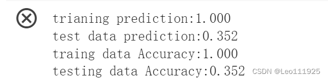
clf = svm.SVC(C=1,kernel='linear',decision_function_shape='ovr') 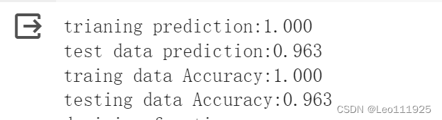
clf = svm.SVC(C=100,kernel='rbf',gamma=0.0001,decision_function_shape='ovr')#0.0001<gamma<10,0.1<C<10 
2、实验结果分析
对于iris数据集和wine数据集而言,数据集的数据量较小,并且存在线性可分性,在用到‘linear’线性核函数的时候可以获得一个识别准确度很高的模型。同时在某些特定参数时‘rbf’高斯核函数,也可得到一个比较好的模型。


 9467
9467


 被折叠的 条评论
为什么被折叠?
被折叠的 条评论
为什么被折叠?
 到【灌水乐园】发言


