使用Python和statsmodels库进行多项式回归分析

题目

下表列出了某城市18位35-44岁经理的年平均收入x1千元,风险偏好度 x2 和人寿保险额y千元的数据,
其中风险偏好度是根据发给每个经理的问卷调查表综合评估得到的,它的数值越大就越偏爱高风险。研究人员
想研究此年龄段中的经理所投保的人寿保险额与年均收入及风险偏好度之间的关系。研究者预计,经理的年均
收入和人寿保险额之间存在着二次关系,并有把握地认为风险偏好度对人寿保险额有线性效应,但对风险偏好
度对人寿保险额是否有二次效应以及两个自变量是否对人寿保险额有交互效应,心中没底。
请你通过表1中的数据来建立一个合适的回归模型,验证上面的看法,并给出进一步的分析。

序号	y	x1	x2
1	196	66.290	7
2	63	40.964	5
3	252	72.996	10
4	84	45.010	6
5	126	57.204	4
6	14	26.852	5
7	49	38.122	4
8	49	35.840	6
9	266	75.796	9
10	49	37.408	5
11	105	54.376	2
12	98	46.186	7
13	77	46.130	4
14	14	30.366	3
15	56	39.060	5
16	245	79.380	1
17	133	52.766	8
18	133	55.916	6

代码

import pandas as pd
import numpy as np
import statsmodels.api as sm
import matplotlib.pyplot as plt

#中文乱码
plt.rcParams['font.sans-serif'] = ['SimHei']

def read_data():
    data = {
        'y': [196, 63, 252, 84, 126, 14, 49, 49, 266, 49, 105, 98, 77, 14, 56, 245, 133, 133],
        'x1': [66.290, 40.964, 72.996, 45.010, 57.204, 26.852, 38.122, 35.840, 75.796, 37.408, 54.376, 46.186, 46.130, 30.366, 39.060, 79.380, 52.766, 55.916],
        'x2': [7, 5, 10, 6, 4, 5, 4, 6, 9, 5, 2, 7, 4, 3, 5, 1, 8, 6]
    }
    return pd.DataFrame(data)

def add_polynomial_terms(df):
    df['x1_squared'] = df['x1'] ** 2
    return sm.add_constant(df)

def fit_polynomial_regression(df):
    model = sm.OLS(df['y'], df[['const', 'x1', 'x2', 'x1_squared']])
    return model.fit()

def save_summary_to_txt(results):
    with open('regression_summary.txt', 'w') as f:
        f.write(results.summary().as_text())

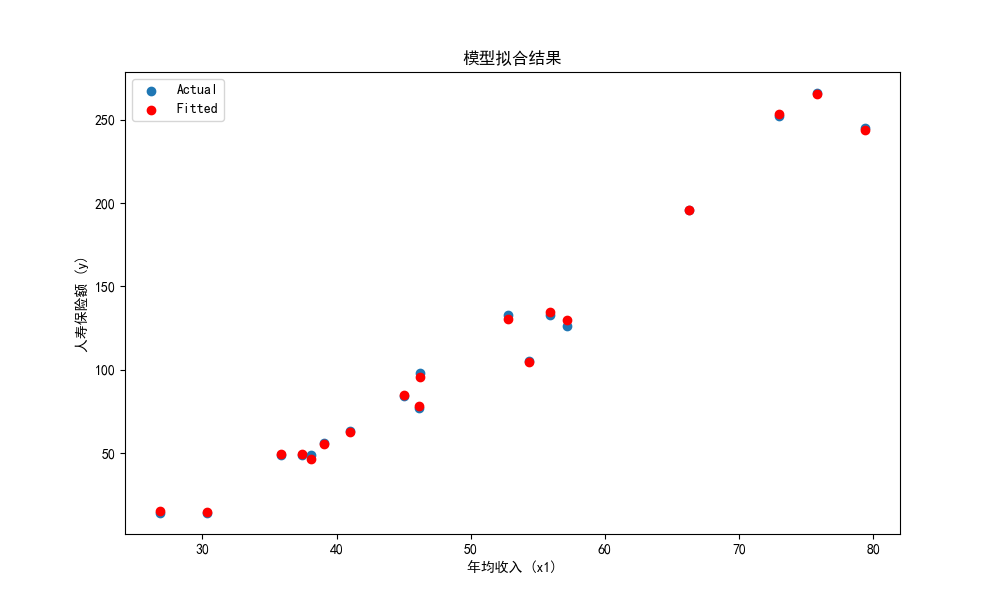
def plot_fitted_values(df, fitted_values):
    plt.figure(figsize=(10, 6))
    plt.scatter(df['x1'], df['y'], label='Actual')
    plt.scatter(df['x1'], fitted_values, color='red', label='Fitted')
    plt.xlabel('年均收入 (x1)')
    plt.ylabel('人寿保险额 (y)')
    plt.title('模型拟合结果')
    plt.legend()
    plt.savefig('模型拟合结果.png')
    #plt.show()

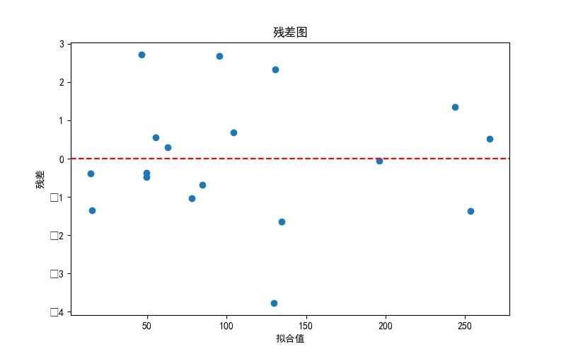
def plot_residuals(fitted_values, residuals):
    plt.figure(figsize=(8, 5))
    plt.scatter(fitted_values, residuals)
    plt.axhline(y=0, color='r', linestyle='--')
    plt.xlabel('拟合值')
    plt.ylabel('残差')
    plt.title('残差图')
    plt.savefig('残差图.png')
    #plt.show()

def save_results_to_txt(results):
    beta_0 = results.params['const']
    beta_1 = results.params['x1']
    beta_2 = results.params['x2']
    beta_3 = results.params['x1_squared']

    with open('regression_results.txt', 'w') as f:
        f.write("Regression Equation:\n")
        f.write(f"y = {beta_0} + {beta_1} * x1 + {beta_2} * x2 + {beta_3} * x1^2 + ε\n\n")
        
        f.write("Regression Summary:\n")
        f.write(results.summary().as_text())

def main():
    # 读取数据
    df = read_data()

    # 添加多项式项和截距项
    df = add_polynomial_terms(df)

    # 拟合多项式回归模型
    results = fit_polynomial_regression(df)

    # 将结果摘要保存为txt文件
    #save_summary_to_txt(results)

    # 打印结果摘要
    print(results.summary())

    # 绘制模型拟合的散点图和拟合线
    plot_fitted_values(df, results.fittedvalues)

    # 绘制残差图
    plot_residuals(results.fittedvalues, results.resid)

    # 将表达式和摘要保存为txt文件
    save_results_to_txt(results)

    print("Results saved to regression_results.txt")

if __name__ == "__main__":
    main()

运行结果

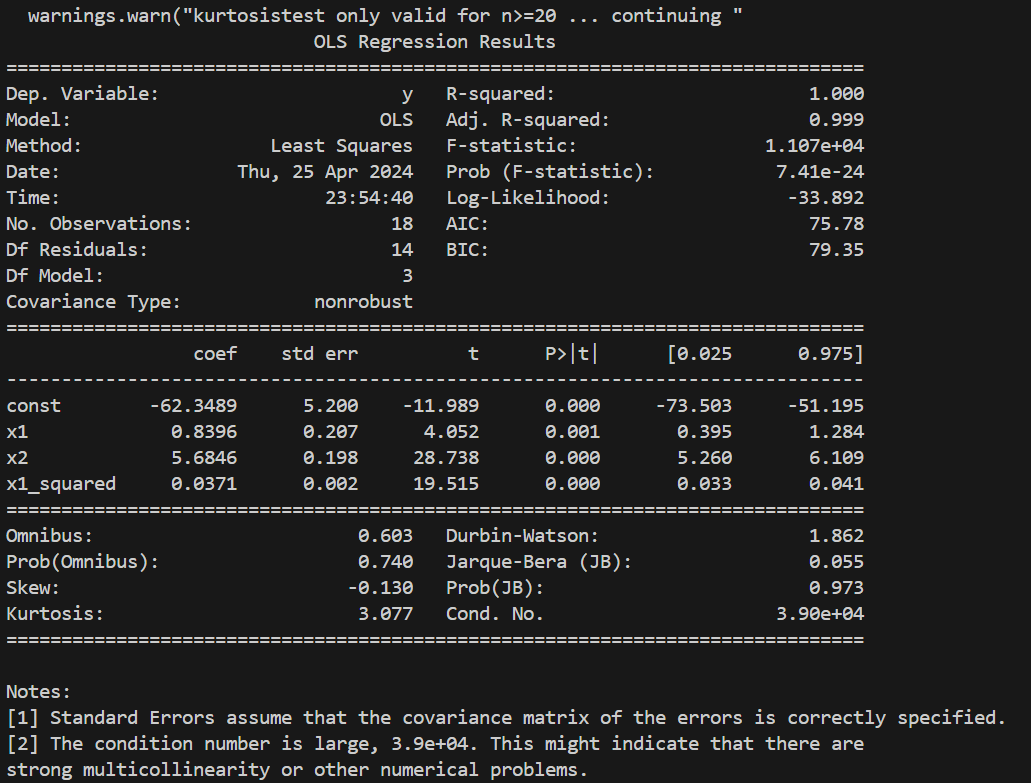
回归方程：

回归方程表明了自变量 x₁、x₂ 和 x₁²（x₁ 的平方项）与因变量 y 之间的关系。

$$y=-62.3489+0.8396x_1+5.6846x_2+0.0371x_1^2$$

结果分析：

• R-squared（R²）：用于衡量回归模型对因变量变异性的解释程度，取值范围为0到1，越接近1表示拟合效果越好。
  • R² = 1.000：表明回归模型完美拟合了数据，自变量能够完全解释因变量的变异性。
• Adj. R-squared（调整 R²）：对 R² 进行调整，考虑了模型中自变量的数量和样本量之间的关系。
  • Adj. R² = 0.999：表示在考虑了自变量数量和样本量后，模型仍然具有很好的拟合效果。
• F-statistic（F统计量）：用于检验模型整体显著性的统计量。
  • F-statistic = 1.107e+04，对应的 p-value 非常小（7.41e-24），表明模型整体显著。
• 残差的正态性检验（Omnibus、Jarque-Bera等统计量）：用于检验残差是否符合正态分布。
  • Prob(Omnibus) = 0.740，Prob(JB) = 0.973：对应的 p-value 较大，表明残差可能符合正态分布。
• Durbin-Watson：用于检验残差是否存在自相关性。
  • Durbin-Watson = 1.862：接近2，表明残差可能不存在一阶自相关性